Feature 1 – What If Analysis Using the Scenario Manager Option
To calculate EMI for a loan, we have 3 parameters, Loan Amount, Interest Rate, and Number of Monthly Payments. You can compare the result of EMI based on the change of these parameters with the Scenario manager tool.
Step 1 – Make a Dataset of the First Scenario
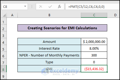
- Create input cells for the Loan Amount, Interest Rate, and Number of Monthly Payments and type.
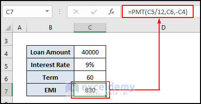
- Use the PMT function to calculate the EMI per month in C8:
=PMT(C5/12,C6,C4,0,0)Formula Breakdown:
Syntax =PMT(rate, nper, PV, [fv], [type])
- Rate = C5/12: D5 represents the annual interest rate of 8%, we divide it by 12 to adjust it for one month.
- NPER = C6 = 60: for 5 years 5*12=60
- PV= C4 = 2000000: the present value is the total loan amount
Read More: How to Do Sensitivity Analysis in Excel
Step 2 – Create the First Scenario
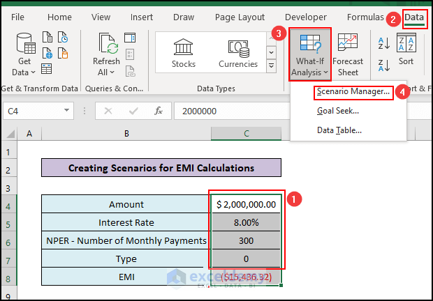
- Select the cells that affect the output EMI. We selected the cell of range C4:C7.
- Go to Data.
- Click on the What–If Analysis option and select Scenario Manager.
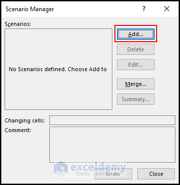
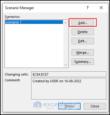
- The scenario manager pop-up window will appear.
- Click on the Add button.
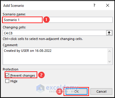
- Another new window will appear named “Add Scenario”.
- Give the name of the Scenario.
- The Changing cells box is already filled with the selected cells range.
- Check that the prevent changes box is marked.
- Press OK.
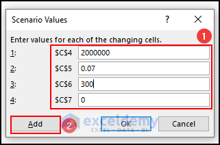
- Another pop-up window will appear and will ask you to give values of the parameter for the new Scenario.
- Insert the values in the respective cells and press OK to save.
Read More: How to Get Sensitivity Report from Solver in Excel
Step 3 – Create More Scenarios
- If you want to add another scenario, click Add.
- Repeat Step 2 to get all the scenarios.
Step 4 – Switch to Another Scenario
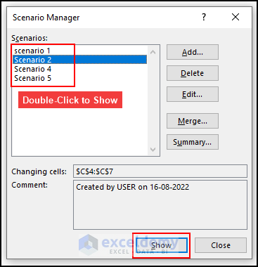
- In the Scenario Manager window, select the scenario that you want to show and click on the Show button below.
- Alternatively, you can simply double–click on the scenario name to show it in the worksheet.
 Read More: How to Perform Sensitivity Analysis for Capital Budgeting in Excel
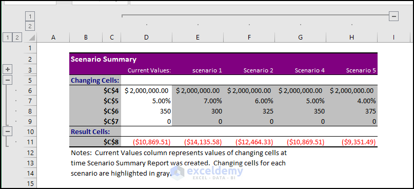
Step 5 – Create the Scenario Summary
- Click on the Summary button in the Scenario Manager
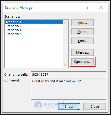
- A pop-up window will appear which will ask you to select the result cell. The result cell will be C8 which is giving the monthly EMI.
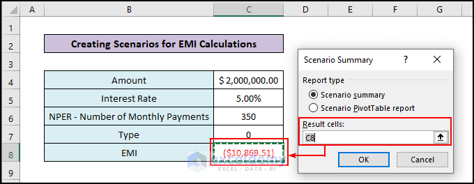
- A new worksheet will be created.
Read More: Sensitivity Analysis for NPV in Excel
Feature 2 – What If Analysis Using the Goal Seek Feature
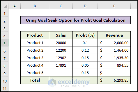
Step 1 – Create the Dataset
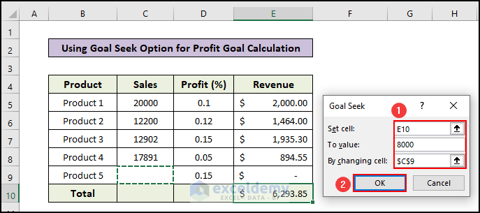
- We have an example dataset where sales of 5 products, profit percentage, and revenue coming from each product are shown. We have listed sales for the first four products but need to determine the required sale amount for product 5 to achieve the target revenue of $8,000.
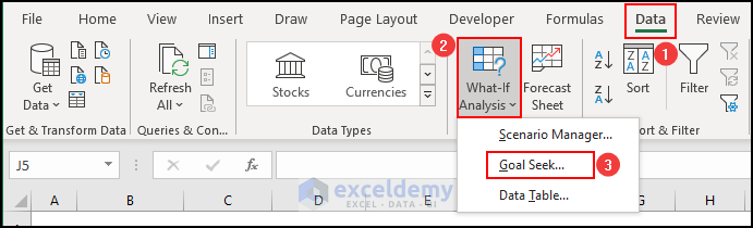
Step 2 – Go to the Goal Seek Feature
- Go to Data.
- Click on What If Analysis.
- Select the Goal Seek feature.
- A new window will appear named “Goal Seek”.
- Select cell E10 as the Set Cell box which is the output.
- Insert the target amount 8000 in the To Value.
- Select cell C9 as the Changing cell.
- Press OK.
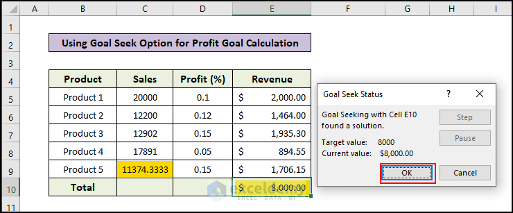
- You’ll get the result.
Read More: How to Delete What If Analysis in Excel
Feature 3 – What If Analysis with the Data Table Option
We’ll create a dataset to calculate the EMI per month as described in the Scenario Manager example.
Case 3.1 – One-Variable Table in a Column
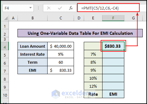
- Create different interest rates in a column and assign cells to get the corresponding EMI value.
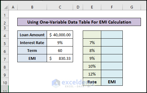
- As our data table is Column-oriented, we have entered the formula in cell F6 to calculate EMI per month in the first row of the EMI column of the data table.
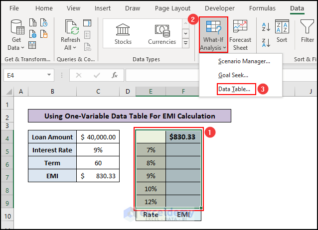
- Select the data table including the cell that contains Present EMI.
- Go to the Data tab in the top Ribbon.
- Click on the What If Analysis option and select Data Table.
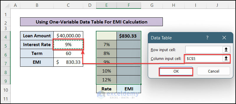
- A new window named Data Table will appear.
- Enter the input cell reference C5 in the Column input cell.
- Press OK.
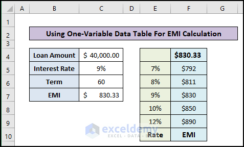
- You will get the column filled with the EMI value respective to the interest rate
Case 3.2 – One-Variable in Row Input
- Insert the present EMI value with the formula in cell B13 which is the First column of the Term row.
- Select the data table including the cell that contains Present EMI.
- Go to the Data tab in the top Ribbon.
- Click on the What If Analysis option and select Data Table
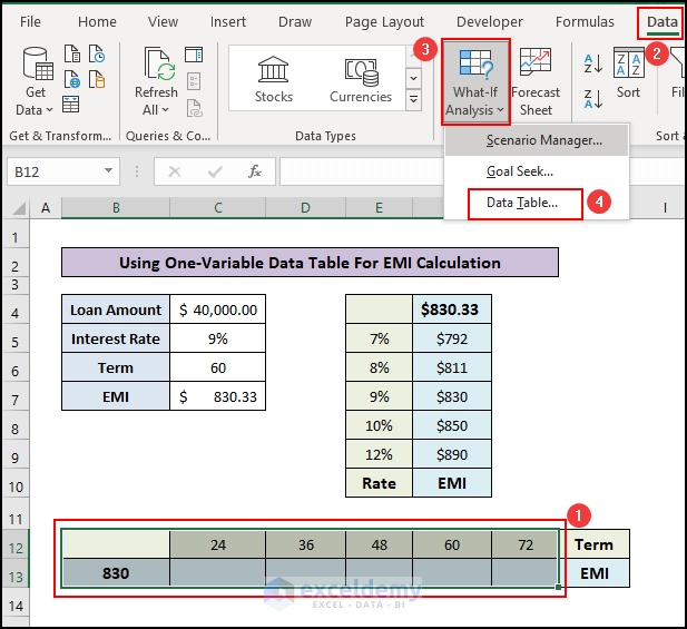
- A new window named Data Table will appear.
- Enter the input cell reference C6 in the Row input cell.
- Press OK.
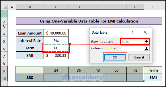
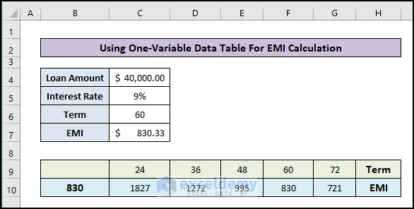
- You will get the column filled with the EMI value respective to the number of terms.
Read More: How to Build a Sensitivity Analysis Table in Excel
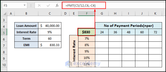
Case 3.3 – Two-Variable Data Table
- Make a data table where you have interest rates along the first column and No. of payment terms along the first row.
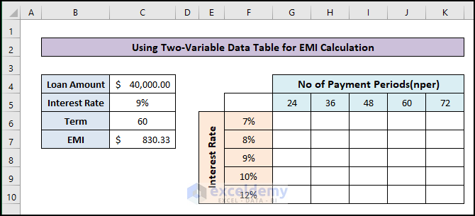
- Insert the present EMI value with the formula in cell F5 which is the cell first row and first column cell of the data table.
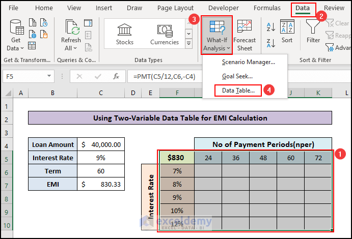
- Select the data table including the cell that contains Present EMI.
- Go to the Data tab in the top Ribbon.
- Click on the What If Analysis option and select Data Table.
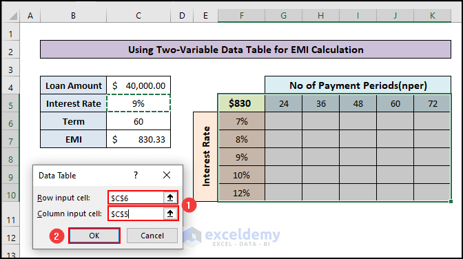
- Anew window named Data Table will appear.
- Enter the input cell reference C6 in the Row input cell.
- Enter the input cell reference C5 in the Column input cell.
- Press OK.
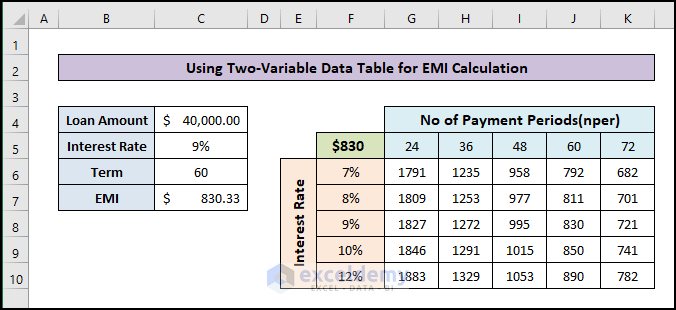
- You will get the column filled with the EMI value respective to the NPER terms and Interest Rates.
Things to Remember
- Use the Scenario Manager feature when you have a certain number of datasets of an irregular pattern.
- Use the Data Table feature when the input variables change in a regular pattern.
- Use the Goal Seek feature to do a back calculation to find an input value using the output formula.
Download the Practice Workbook
Related Article
<< Go Back to What-If Analysis in Excel | Learn Excel
Get FREE Advanced Excel Exercises with Solutions!
