How to Use What-If Analysis in Excel (Definition and Types)

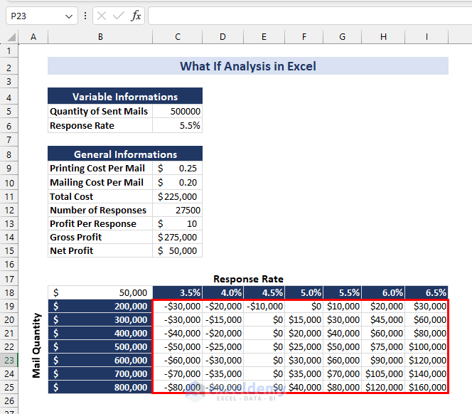
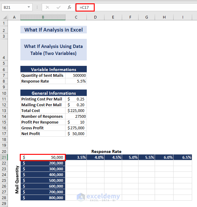
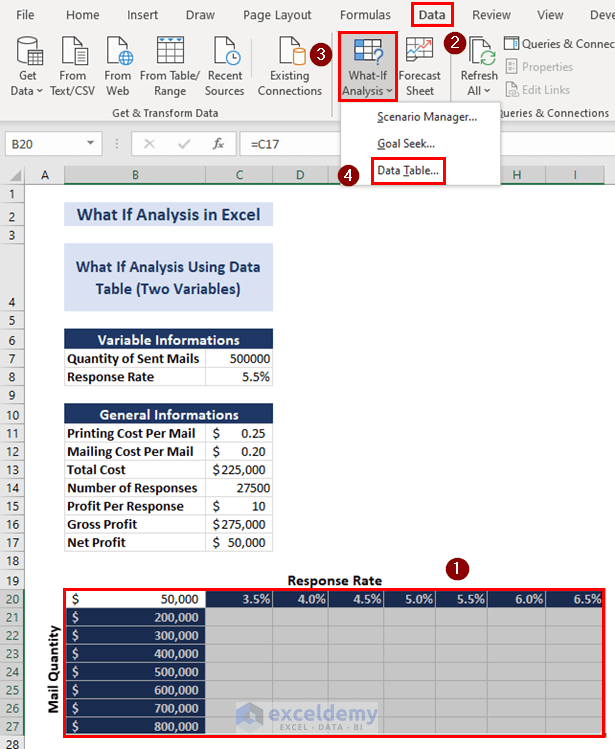
In the following dataset, we have a two-variable what-if analysis on a direct mail profit model. One variable is the response rate, which varies through the columns, and another is the mail quantity, which varies through the rows. The corresponding values of the net profits are visible in the table.

What Is a What-If Analysis in Excel?

A What-If Analysis in Excel refers to exploring various scenarios by changing input values in a spreadsheet to see how they affect the outcomes. It helps users analyze different possibilities and make informed decisions by observing the impact of changes on data trends within Excel models. There are 3 different tools in What-If Analysis.

1. Scenario Manager: Scenario Manager helps create a report when one or more values in the dataset are changed. This report shows how the result will change upon changing an input value.
2. Goal Seek: The Goal Seek feature helps when someone knows the final value they want and needs to know how to change the input value to achieve the desired result.
3. Data Table: The Data Table feature table helps to create a table with different scenarios depending on the variable change.

How to Use a Scenario Manager for What-If Analysis in Excel

Example 1: Tax Rate

Steps:

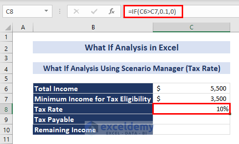
• Enter the following formula in cell C8:

• Press ENTER. The tax rate is calculated based on the total income.

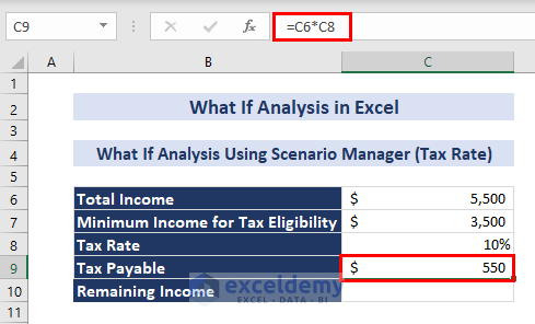
• Enter the following formula in cell C9:

• Press ENTER. The tax payable amount is calculated.

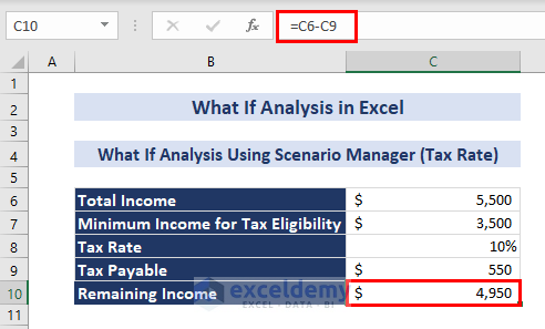
• Enter the following formula in cell C10:

• Press ENTER. The remaining income after tax deductions is calculated.

To perform the what-if analysis by varying the tax rate and observing changes in the tax payable:

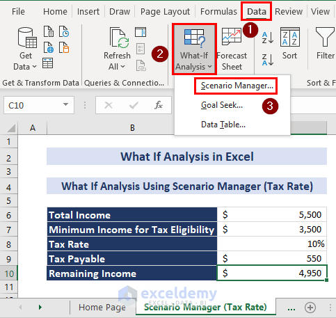
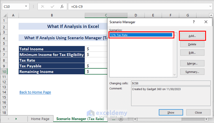
• Go to the Data tab => What-If Analysis inside the Forecast group => Scenario Manager…

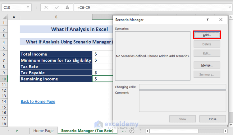
• Click on Add… inside the Scenario Manager dialogue box.

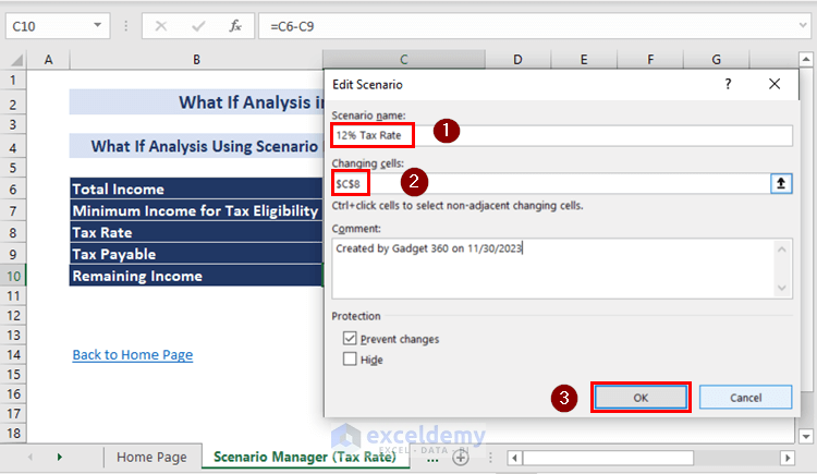
• Inside the new dialogue box named Edit Scenario, insert the Scenario name as 12% Tax Rate, and insert $C$8 as the location of the Changing cells.
• Click on OK.

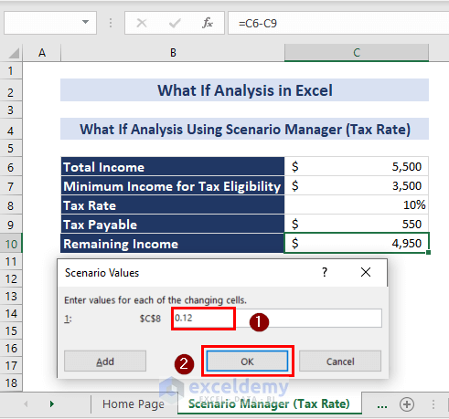
• Inside the Scenario Values dialogue box, under Enter values for each changing cell, type 0.12, as we named the scenario 12% Tax Rate.
• Click on OK.

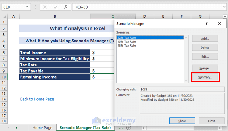
• Following the same procedure, we can add as many scenarios as we want. Before adding a new scenario, click on add.

Here, we have added three scenarios in total.

• Click on Summary…

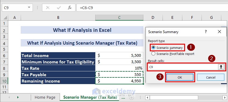
• Inside the Scenario Summary dialogue box, select Scenario Summary.
• Type C9 under Result cells, and click OK.

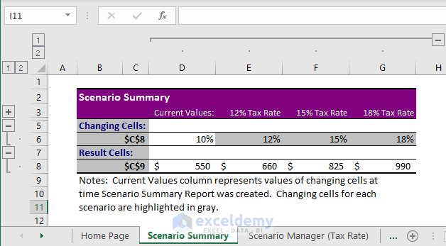
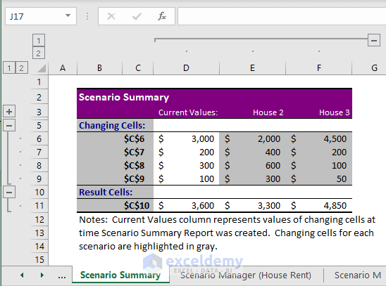
The result of the what-if analysis will now appear on a new sheet in the form of a table titled “Scenario Summary”. There, you can see the changed values of tax payable with varying tax rates.

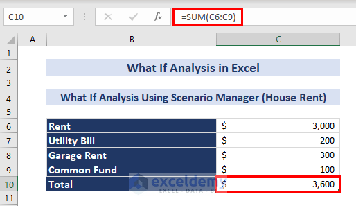
Example 2: House Rent

Steps:

• To calculate the total rent of house 1, enter the following formula in cell C10:

• Press ENTER.

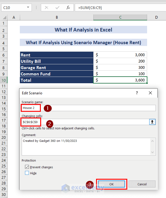
• Go to the Scenario Manager and click on Add as before.
• Write House 2 under the Scenario name inside the Edit Scenario dialogue box.
• Select a range of cells, such as $C$6:$C$9, instead of a single cell under Changing cells; multiple cell values will now change the total rent value.
• Click OK.

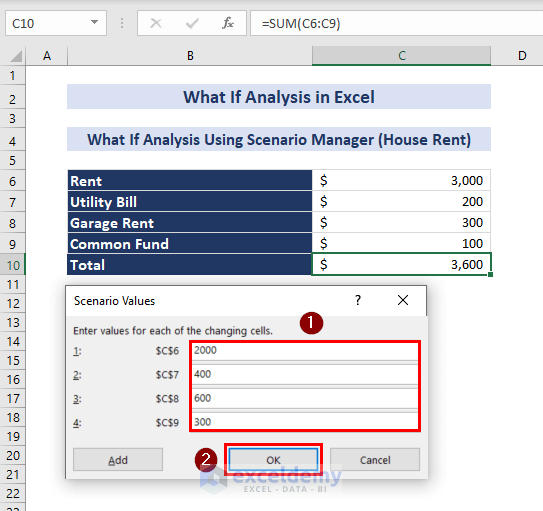
• Input the scenario values inside the respected fields for House 2 inside the Scenario Values dialogue box.
• Click OK.

• Follow the process for adding new scenarios and getting the summary from Example 1. Specify the Result cells: as C10 in this case.
• Click OK.

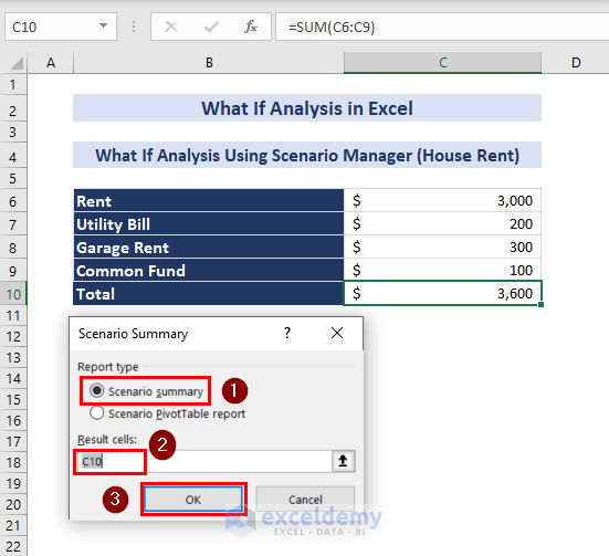
The result of the what-if analysis will now appear in a new sheet as a table, titled “Scenario Summary,” as before. There, you can see the values of the total rents of 3 houses with varying rent parameters.

How to Use Goal Seek for What-If Analysis in Excel

Example 1: Profit Goal

Steps:

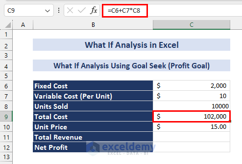
• Enter the following formula inside cell C9:

• Press ENTER. The total cost of the product is calculated based on the given data.

• To calculate the total revenue, enter the following formula in cell C11:

• Press ENTER.

• To calculate the net profit, enter the following formula in cell C12:

• Press ENTER.

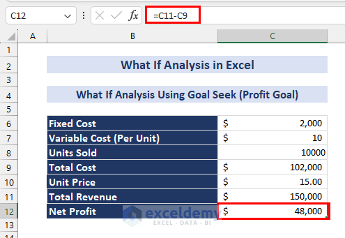
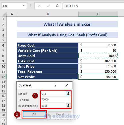
Suppose we aim to increase our net profit from $48000 to $70000. Now we will find out how many units of product we need to sell if we want to make $70000 in net profit, keeping all other parameters constant.

• Go to Data tab => What-If Analysis from Forecast group => Goal Seek…

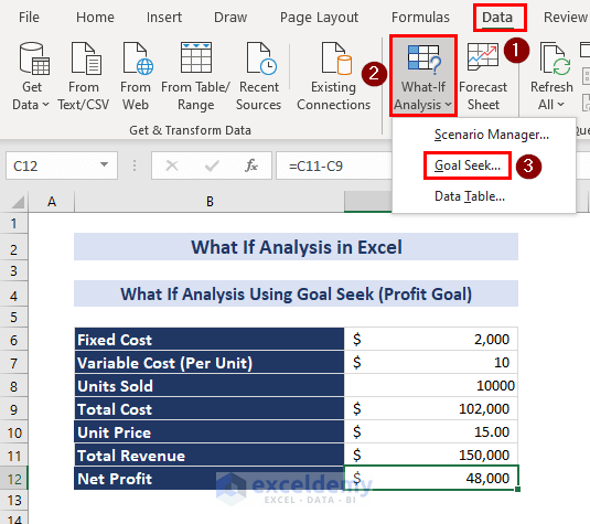
A dialogue box named Goal Seek will appear.

• Beside the Set cell: type the cell address of the net profit value (in this case, C12).
• Beside To value: type the target value (in this case, 70000).
• Besides changing cell: type the cell address of the number of products sold (in this case, $C$8).
• Click on OK.

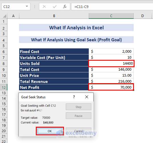
A dialogue box will appear stating the current and previous values of net profit. The quantity of units sold changes according to the new net profit in the data table.

• Click on OK to keep the changes in the data table.

Example 2: Passing Score

Steps:

• Enter the following formula in cell C12:

• Press ENTER. The total marks obtained by the student is calculated.

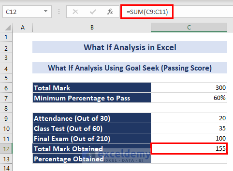
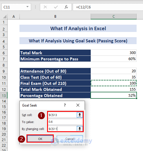
• Enter the following formula in cell C13:

• Press ENTER. The percentage of the obtained marks is currently 52%.

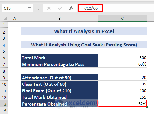
Our goal is to achieve 60% marks to pass the course, and we will evaluate the minimum marks that are required to score in the final exam to achieve that percentage, given that the other parameters are constant.

• To do that, go to the Goal Seek… feature as before.
• In the Goal Seek dialogue box, enter the following information:

Set cell: $C$13
To value: 0.6
By changing cell: $C$11

• Click on OK.

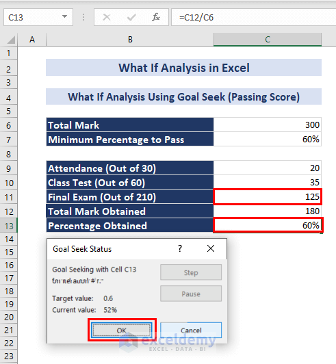
We can see that the minimum mark required to achieve a passing percentage in the final exam is 125.

• Click OK to keep the changes.

How to Use Data Tables for What-If Analysis in Excel

Example 1: One Variable Sensitivity Analysis

Steps:

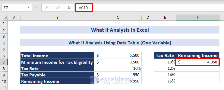
• Create a second data table on the right side of the previous one, with two columns: one for the varying tax rates and another for the corresponding remaining incomes, as shown in the image below. Also, enlist the tax rates for which we want to know the remaining incomes.
• Enter the following formula in cell F7:

• Press ENTER.

• Select the range E7:F10 and click on Data tab => What-If Analysis inside Forecast group => Data Table…

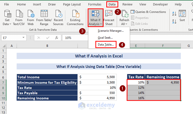
• In the dialogue box named Data Table, select the cell $C$8 that contains the current tax rate beside the Column input cell:
• Click on OK.

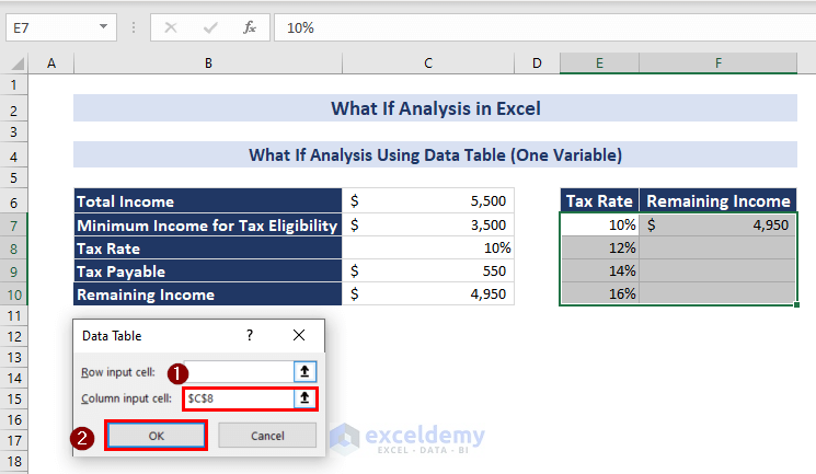
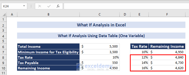
The remaining incomes for the mentioned tax rates are visible inside the corresponding cells.

Example 2: Two-Variable Sensitivity Analysis

Steps:

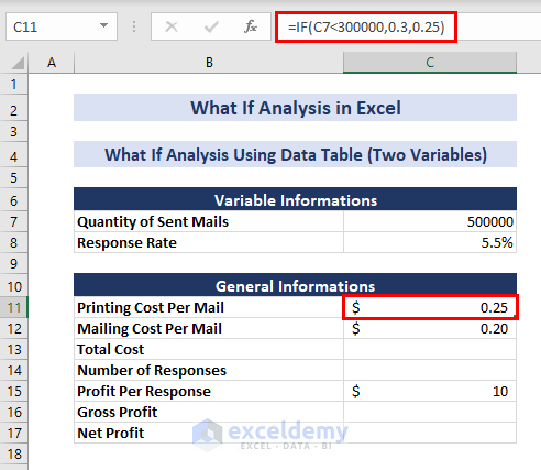
• Enter the following formula in cell C11:

• Press ENTER. This formula generates the printing cost per mail as $0.3 if the total number of mail to be printed is below 300000 and $0.25 if the number is greater than 300000.

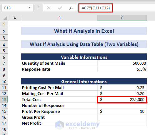
• Enter the following formula in cell C13:

• Press ENTER. This will calculate the total cost of sending the mail.

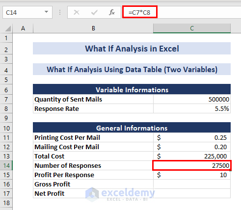
• Enter the following formula in cell C14:

• Press ENTER. This will calculate the number of responses received after sending the mail.

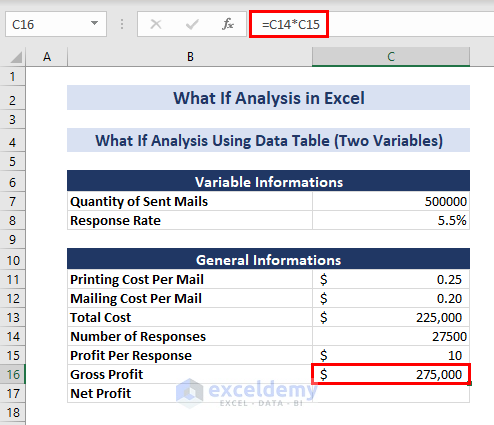
• To calculate the gross profit, enter the following formula in cell C16:

• Press ENTER.

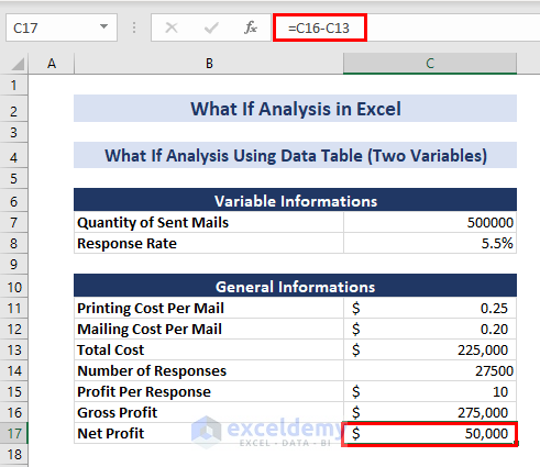
• Enter the following formula in cell C17:

• Press ENTER. The net profit for the initial conditions is calculated.

Now, to create a two-variable data table in Excel for performing sensitivity analysis on this data model:

• Create a new data table that will accommodate the varying response rates as columns and mail quantities as rows, as shown in the image below.
• Enter the following formula in cell B21:

• Press ENTER.

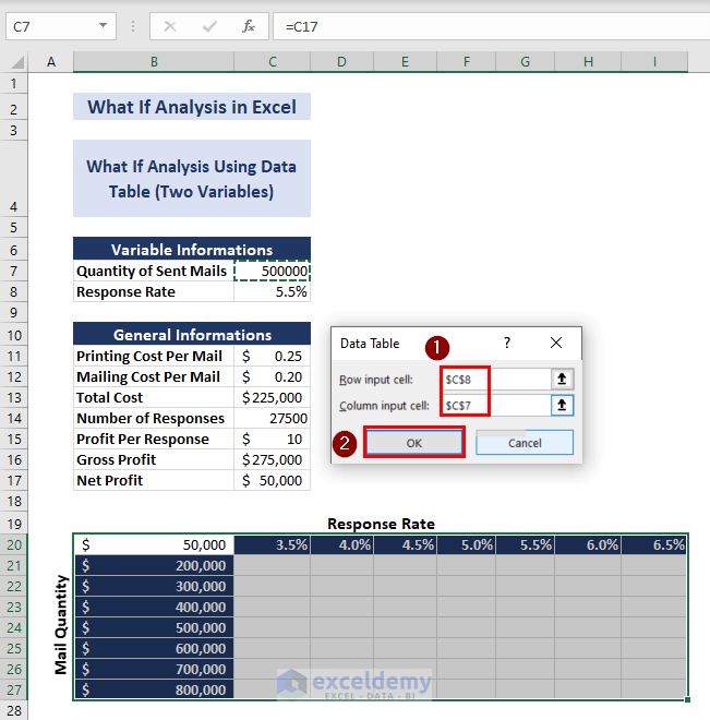
• Select the range B20:I27 and click on Data tab => What-If Analysis inside Forecast group => Data Table…

• Enter the following information in the Data Table dialogue box:

Row input cell: $C$18
Column input cell: $C$7

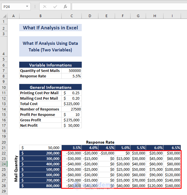
• Click on OK.

The net profits for the mentioned mail quantities and response rates are visible inside the corresponding cells. The negative net profit values explain that losses take place under those corresponding mail quantities and response rates instead of any profit.

Example 3: Three Variable Sensitivity Analysis

Steps:

• Create another table for the third variable, as shown in the image below (Range E6:F12).
• Create a drop-down list inside cell E7 containing the varying profit per response value.
• Enter the following formula in cell C15:

• Press ENTER.

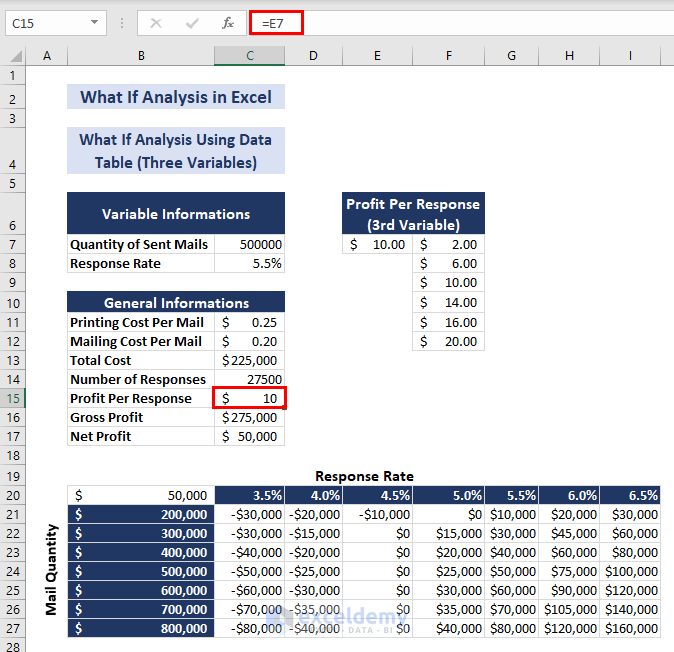
Our three-variable data table is now ready for what-if or sensitivity analysis.

Choose any profit per response from the drop-down list in cell E7 and observe the dynamic changes in the corresponding net profits.

How to Fix If Goal Seek Is Not Working in Excel

1. Recheck Goal Seek Parameters

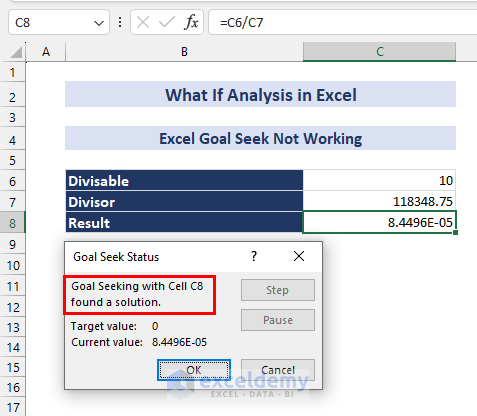
Make sure the cell you’re setting refers to a cell with a formula. Also, ensure that the cell you are changing refers to a cell with no formula but value. Then, check if the formula in that cell depends on the changing cell, either directly or indirectly.

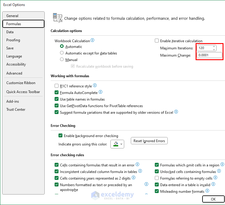
2. Adjust Maximum Iterations

Follow the steps below to solve the problem:

• Go to File => Options => Formulas
• Make changes in the following parameters:

Maximum Iterations: If you want Excel to explore more possible solutions, raise this number.

Maximum Change: Lower this number if your formula needs to be more precise. For instance, if you’re working with a formula where the input should be 0, but Goal Seek stops at 0.1, adjusting the maximum change to 0.0001 can help solve the problem.

You can see that this time, Goal Seek Status shows that a solution was found.

3. Avoid Circular References

To ensure Goal Seek or any Excel formula functions correctly, the formulas involved mustn’t rely on each other. Circular references occur when a formula refers to its cell directly or indirectly, creating a loop. Avoiding such interdependencies helps prevent errors and ensures the accurate execution of calculations in Excel.

Here, we have demonstrated and solved a problem related to the Goal Seek feature. But if you face a problem with the what-if analysis data table not working in Excel while using the data table feature, you can visit the linked article.

 Download the Practice Book

What-If Analysis in Excel: Knowledge Hub

<< Go Back to Learn Excel