How to Build a Sensitivity Analysis Table in Excel (One-Variable and Two-Variable)

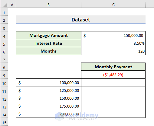
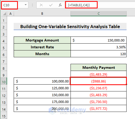
This guide will show you how to build sensitivity analysis tables in Excel, looking at both single factors and two factors at once. To illustrate, we’ll use the following dataset as an example. For instance, we have a Mortgage Amount, Interest Rate, and Months. In the One-Variable case, we’ll consider 5 different mortgage amounts. And in the Two-Variable case, we’ll take 3  different values for months along with the 5 mortgage amounts. In cell C9, we input the formula:

The PMT function determines the loan amount for a fixed interest rate, time period, and present value of the mortgage.

1. Build One Variable Sensitivity Analysis Data Table in Excel

STEPS:

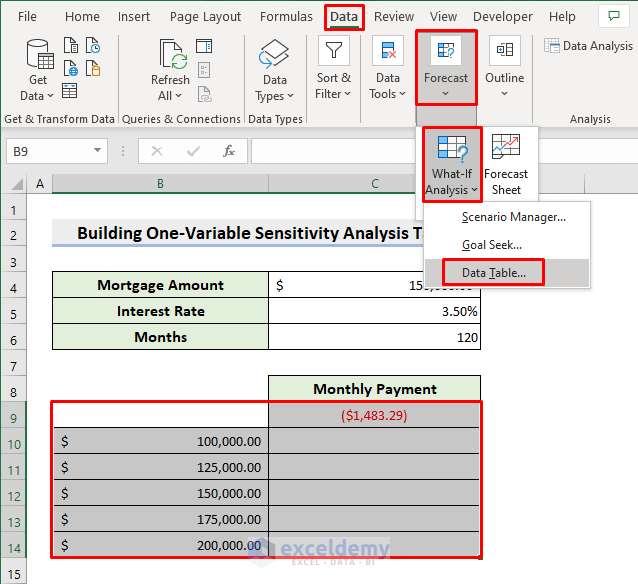
• Select the cell range B9:C14.
• Go to Data ➤ Forecast ➤ What-If Analysis ➤ Data Table.

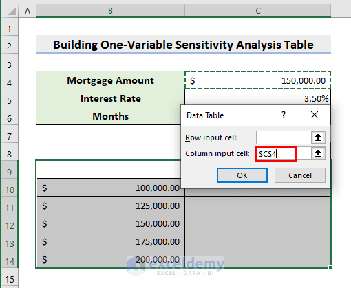
• In the Data Table window, select the cell that has the variable you want (this is cell C4 in our example) as the Column input cell.
• Hit OK.

• Excel will generate different monthly payment amounts based on the different loan amounts you entered.

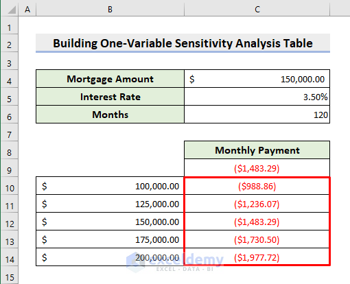
• Click any cell in the generated result range (C10:C14).
• You’ll see the same formula applied to all the output values.

Read More: How to Use What If Analysis in Excel

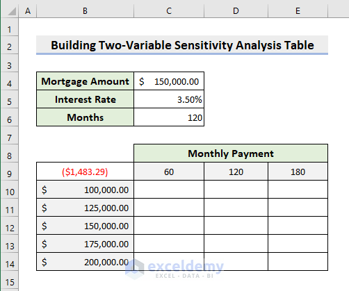
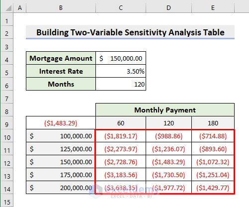
2. Create Excel Two-Variable Sensitivity Analysis Table

In this example, we’ll arrange our dataset to consider the two variables. We’ll take 3 different time periods (60 months, 120 months, and 180 months) to pay back the mortgage amount. Here, 5 different values for the mortgage will be considered as well. We’ll move the formula in cell C9 for calculating the loan to cell B9.

STEPS:

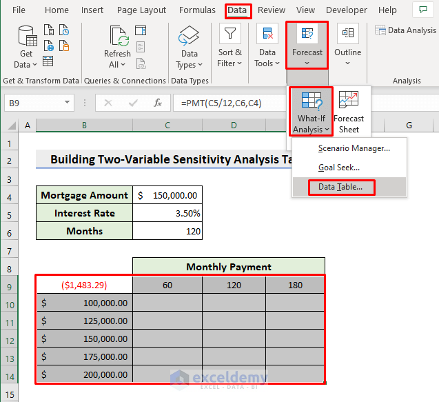
• Choose the range B9:E14.
• Select Data ➤ Forecast ➤ What-If Analysis ➤ Data Table.

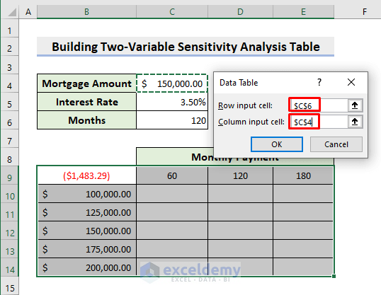
• In the Data Table window, choose C6 in the Row input cell.
• Select cell C4 as the Column input cell.
• Hit OK.

• It will generate the sensitivity analysis data table as shown below.

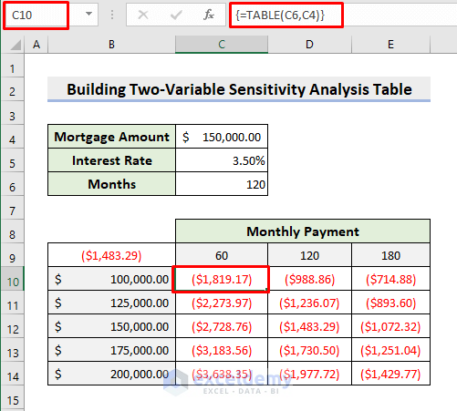
• Select any cell in the output range.
• You’ll see that the same formula is behind all the outputs.

Read More: How to Perform Sensitivity Analysis for Capital Budgeting in Excel

Things to Remember

• Any changes in the input data will result in changes in the final calculation of the output data. For example, if you change the interest rate, the monthly payment amounts will get modified too.
• You can’t edit or delete parts of the results table that Excel automatically fills in. You’ll get a warning message if you try to do so.
• When setting up a two-variable table, double-check that you’ve chosen the right cells for the row and column variables. Otherwise, it’ll result in a big error.

Download Practice Workbook

Related Articles

• How to Get Sensitivity Report from Solver in Excel
• Sensitivity Analysis for NPV in Excel
• How to Do IRR Sensitivity Analysis in Excel
• What-If Analysis in Excel with Example
• What If Analysis Data Table Not Working
• How to Delete What If Analysis in Excel

<< Go Back to What-If Analysis in Excel | Learn Excel