How to Do IRR Sensitivity Analysis in Excel (with Detailed Steps)

Step 1: Input Basic Particulars

Type ‘IRR Sensitivity Analysis’ in some merged cells in a larger font size. That will make the heading more attractive.
Type the required headline fields for your data.
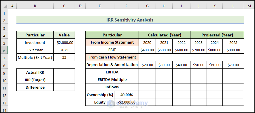
After completing the heading, enter the following Particular, Value, Calculated (Year), and Projected (Year) columns.
Enter the EBIT value which you will obtain from the income statement.
Type the depreciation and amortization value.

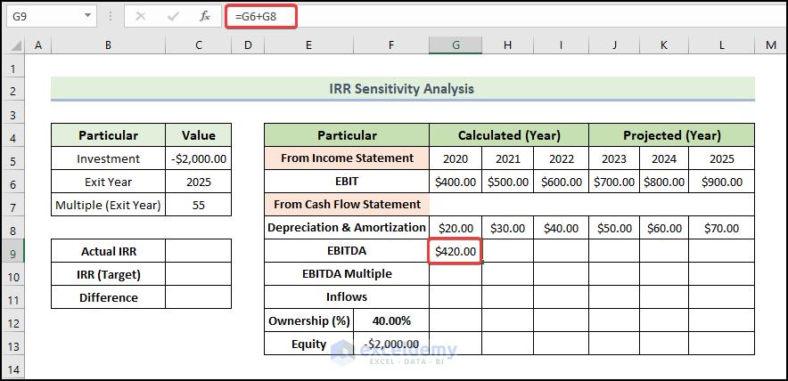
You will get the EBITDA by adding the EBIT with depreciation and amortization.

input basic particulars to Do IRR Sensitivity Analysis in Excel

Step 2: Evaluate EBITDA and Equity Value

To calculate the EBITDA, type the following formula:

=G6+G8

Press Enter.

You will get the EBITDA for the year 2020.

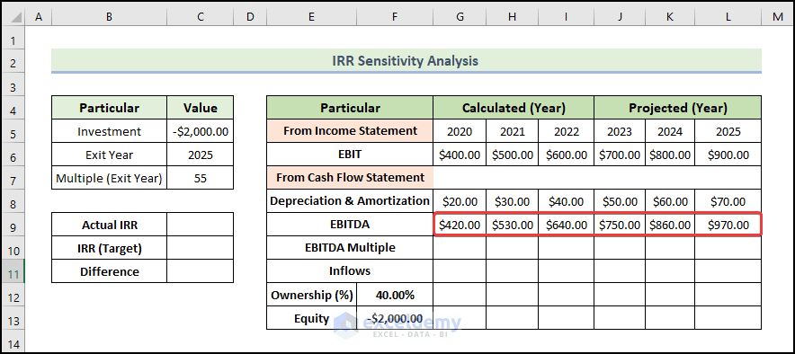
Drag the Fill Handle icon to the right to fill other cells with the formula.

You will get the other year’s EBITDA.

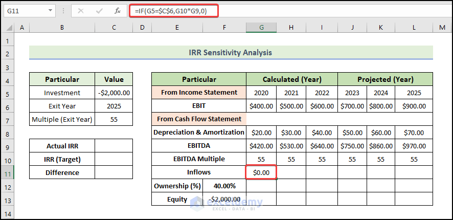
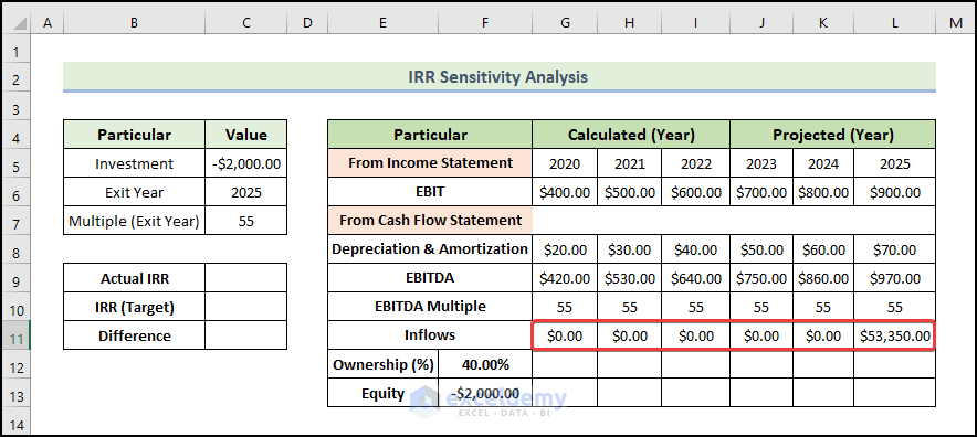
Input the EBITDA Multiple as shown below.
To calculate the Inflows, type the following formula:

=IF(G5=$C$6,G10*G9,0)

Press Enter.

You will get the Inflows for the year 2020.

Drag the Fill Handle icon to the right to fill other cells with the formula.

You will get the other year’s Inflows.

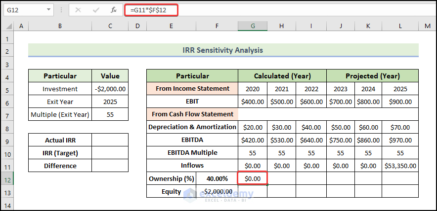
To calculate the Ownership, type the following formula:

=G11*$F$12

Press Enter.

You will get the Ownership for the year 2020.

Drag the Fill Handle icon to the right to fill other cells with the formula.

You will get the other year’s Ownership.

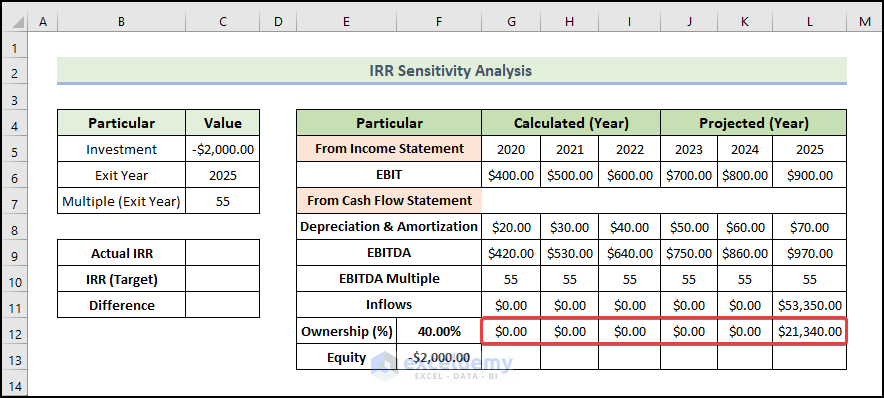
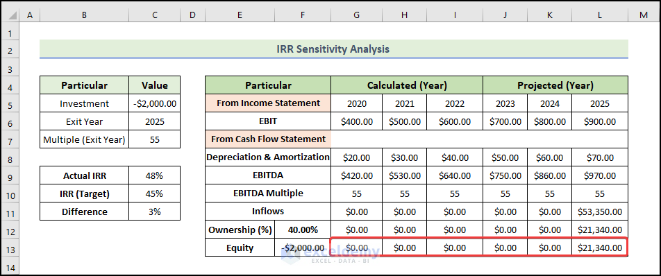
To find out the equity value, enter the ownership value.

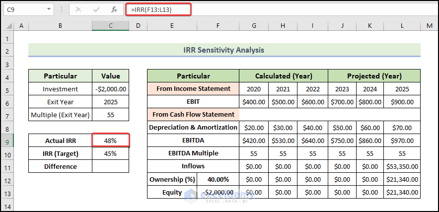
Step 3: Calculate IRR

To calculate the IRR, type the following formula:

=IRR(F13:L13)

Press Enter.

You will get the IRR value.

We assume that our target IRR value is 45%.

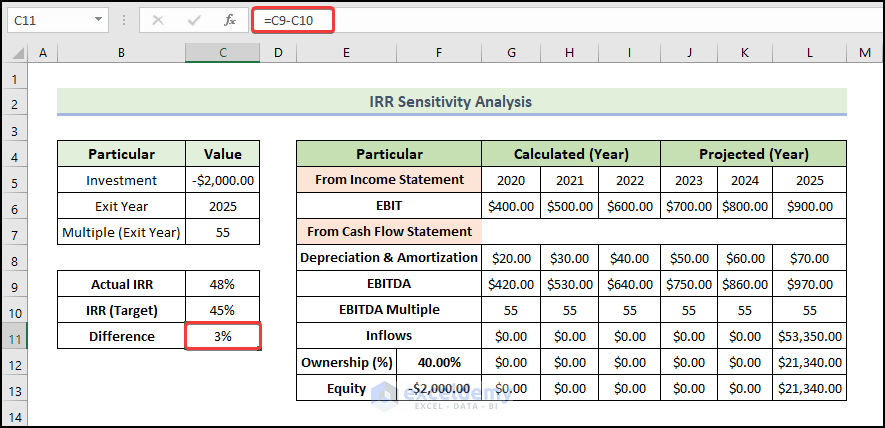
To calculate the Difference, type the following formula:

=C9-C10

Press Enter.

You will get the 3% difference between the actual and target IRR.

Note:

To calculate the IRR value, we can also use the MIRR and XIRR functions and the conventional formula.
The conventional formula is the NPV formula described at the article’s start. In this formula, you have to find the value of IRR by trials for which the summation of all the cash flow values gets closest to zero (NPV to zero).

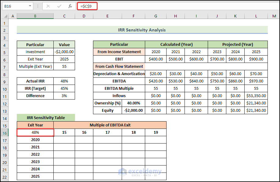
Step 4: Create an IRR Sensitivity Table

Enter the actual IRR value into cell B16 using the following formula:

=$C$9

Press Enter.

Select the range of the cells as shown below.
Go to the Data tab.
Select What-If-Analysis and select the Data Table.

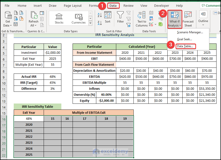
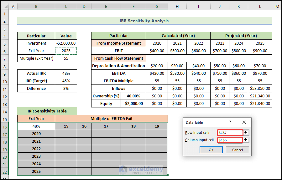
The Data Table window will appear.
Insert the desired cells into the Row input cell and the Column input cell as in the below image.
Click OK.

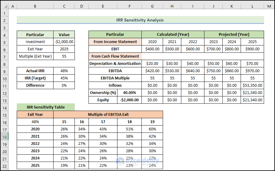
You will get the following IRR sensitivity table. If you change input values in a worksheet, the values calculated by a data table change too.

Note:

You cannot delete or edit a portion of a data table. If you select a cell in the data table range and edit it accidentally, the Excel file will prompt a warning message, and you can’t save, change, or even close the file anymore. The only way that you can close it is by ending the task from task management. It means your time and effort will be wasted if you did not save the file before making that mistake.
The automatic calculation is enabled by default, and that’s the reason why any change in the inputs can cause all the data in the data table to be recalculated. This is a fantastic feature. However, sometimes we’d like to disable this feature, especially when the data tables are large and automatic recalculation is extremely slow. In this situation, how can you disable automatic calculation? Just click the File tab on the ribbon, choose Options, and then click the Formulas tab. Select Automatic Except For Data Tables. Now all your data in the data table will be recalculated only when you press the F9 (recalculation) key.

Things to Remember

✎ No further operation is allowed in a data table as it has a fixed structure. Inserting or deleting a row or column will show a warning message.

✎ The data table and the input variables for the formula must be in the same worksheet.

✎ Do not mix up your row input and column input cells when making a data table. This kind of mistake can result in a big error and nonsensical results.