Method 1 – Sensitivity Analysis with One-Variable Data in Excel
Steps:
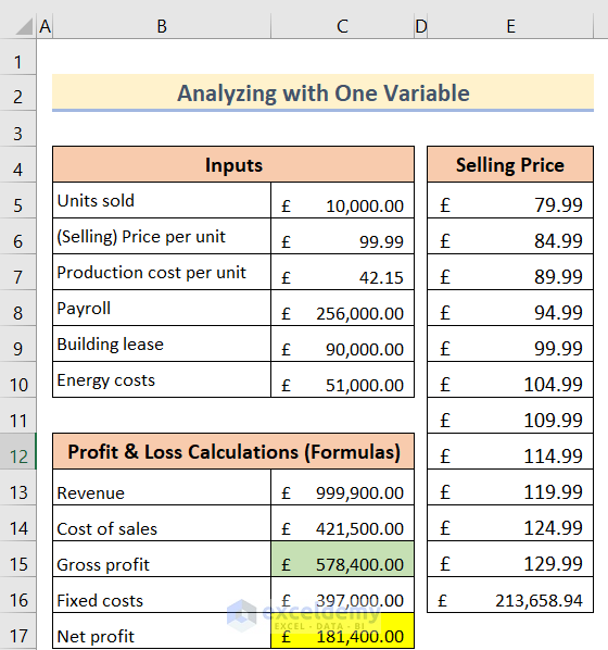
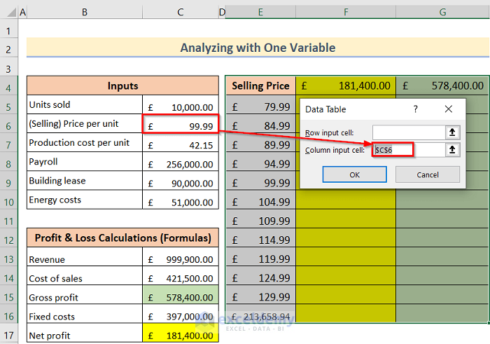
- Create a dataset like in the image below and mark the Gross profit and Net profit cells with the desired color (manually). The cells in Formulas need to be referencing the cells from Inputs.
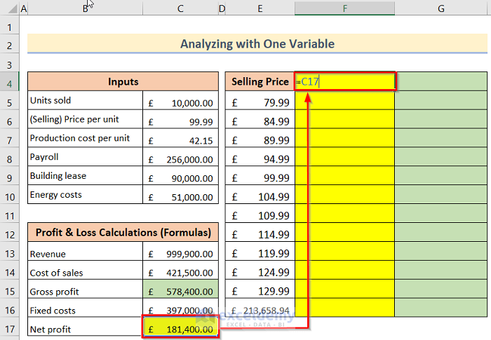
- Reference the Net profit value from the table in cell F4.
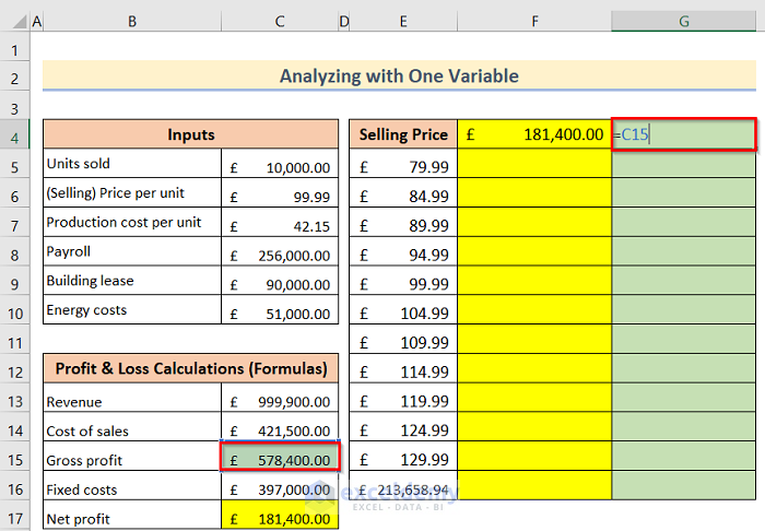
- Reference the Gross profit value in cell G4.
- Select the whole data table you want to analyze.
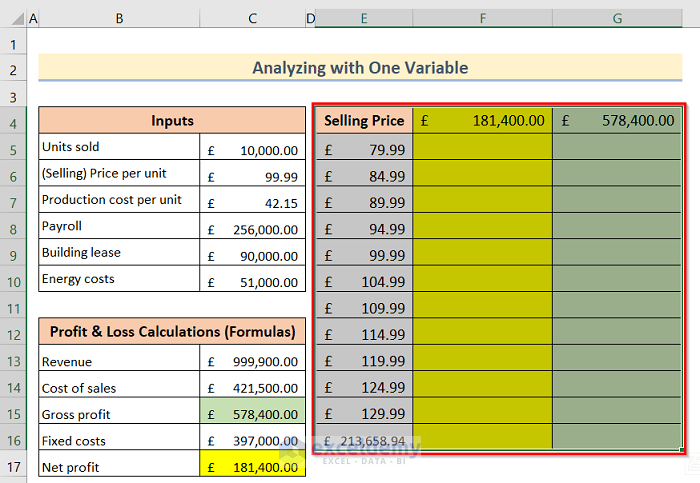
- Go to Data > Forecast > What-If Analysis option.
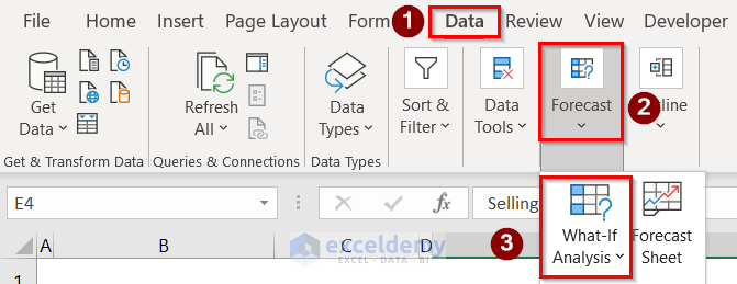
- The Data Table dialog box will open on the screen. Select the variable cell (in this case cell $C$6) in the Column input cell option.
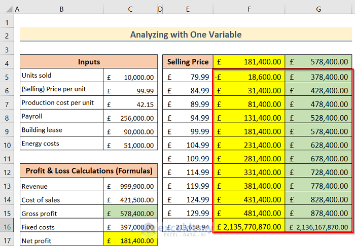
- The table will autofill.
Read More: How to Use What If Analysis in Excel
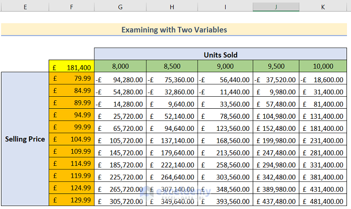
Method 2 – Perform Sensitivity Analysis with a Two-Variable Data Table
Let’s consider two variables: Units Sold and Selling Price. The two-variable data table will show different values for a single result (such as Net Profit) as the variables change.
Steps:
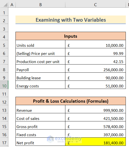
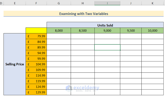
- Create a proper dataset and mark the Net profit value as the one being analyzed.
- Create another data table like the below image. The two variables (Units Sold and Selling Price) should be marked.
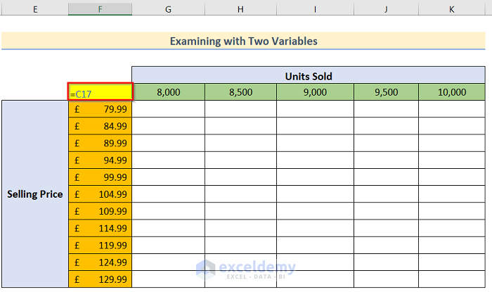
- Reference the Net profit value from the first table (cell C17) into the F5 cell of this table.
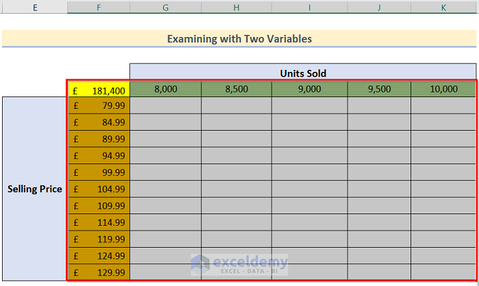
- Select the data table portion you want to use for analysis.
- Go to Data > Forecast > What-If Analysis options.

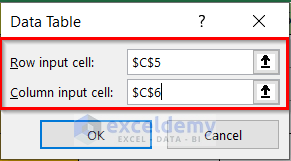
- Insert the desired cells in the Row input cell and the Column input cell with absolute references (see image below) and press OK.
- The table will populate.
Read More: How to Build a Sensitivity Analysis Table in Excel
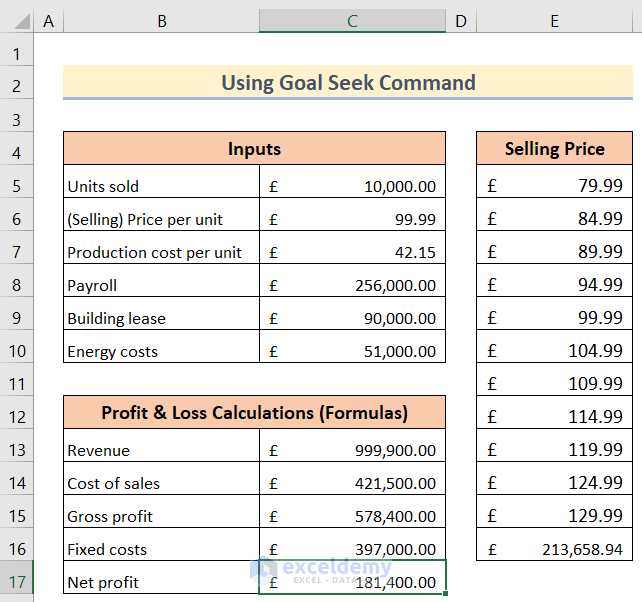
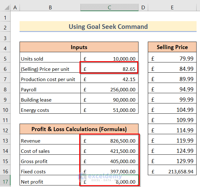
Method 3 – Using Goal Seek Command for Sensitivity Analysis to Set a Variable
Steps:
- Construct a dataset below (use the download sample).
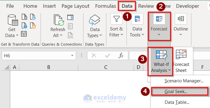
- Go to Data > Forecast > What-If Analysis > Goal Seek.
- In the Goal Seek dialog box, select cell C17 in the Set cell option (the cell you want to change). Then choose 8000 (the desired value you want to achieve) in the To Value option and select cell C6 (the cell you want to use as the variable) and press OK.
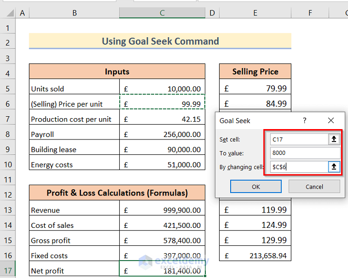
- The Goal Seek formula will adjust cell C6 based on the expected value in C17.
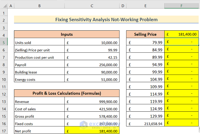
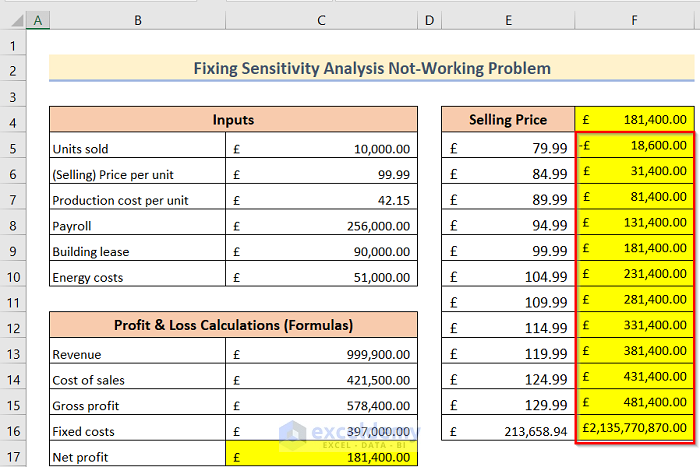
How to Fix “Sensitivity Analysis Not Working in Excel”
Steps:
- Identify if you have a problem like the below image.
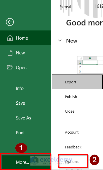
- Select the File tab.

- Go to More…>Options. The Excel Options dialog box will open on the screen.
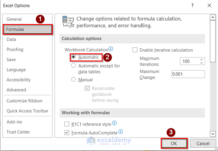
- Select the Formulas tab, then choose the Automatic option in the Calculations options and press OK.
- This should fix the table.
Read More: What If Analysis Data Table Not Working
Download Practice Workbook
You can download the practice workbook from here.
Related Articles
- How to Perform Sensitivity Analysis for Capital Budgeting in Excel
- How to Get Sensitivity Report from Solver in Excel
- Sensitivity Analysis for NPV in Excel
- How to Do IRR Sensitivity Analysis in Excel
- How to Delete What If Analysis in Excel
<< Go Back to What-If Analysis in Excel | Learn Excel
Get FREE Advanced Excel Exercises with Solutions!
