How to Highlight Highest Value in Excel (3 Quick Ways)

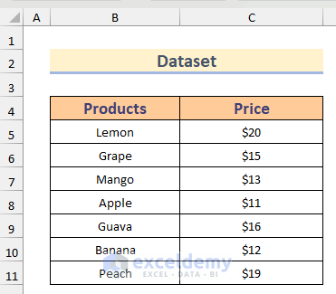
Method 1 – Use Conditional Formatting to Highlight the Highest Value in a Column in Excel

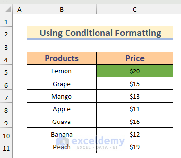
The sample database contains fruit prices in 2 columns and 8 rows. We’ll use Conditional Formatting to highlight the highest value in the range.

Steps:

• Select the data range.
• Go to Home, select Conditional Formatting, and choose New Rule.
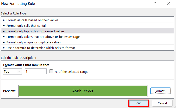
• A dialog box named New Formatting Rule will open up.

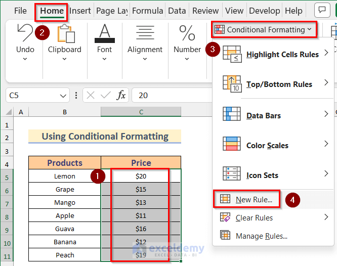
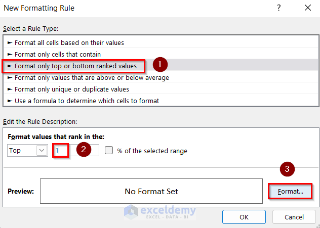
• Choose Format only top or bottom ranked values from the Select a Rule Type box.
• Put 1 in the box under the Format values that rank in the option.
• Press the Format button.
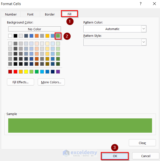
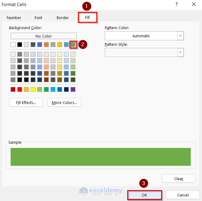
• A dialog box named Format Cells will appear.

• Choose your desired highlight color from the Fill tab and press OK.

• Press OK to close the Formatting Rule window.

• The highest value is highlighted with green color.

Read More: How to Highlight Lowest Value in Excel

Method 2 – Apply Conditional Formatting to Highlight the Highest Value in Each Row in Excel

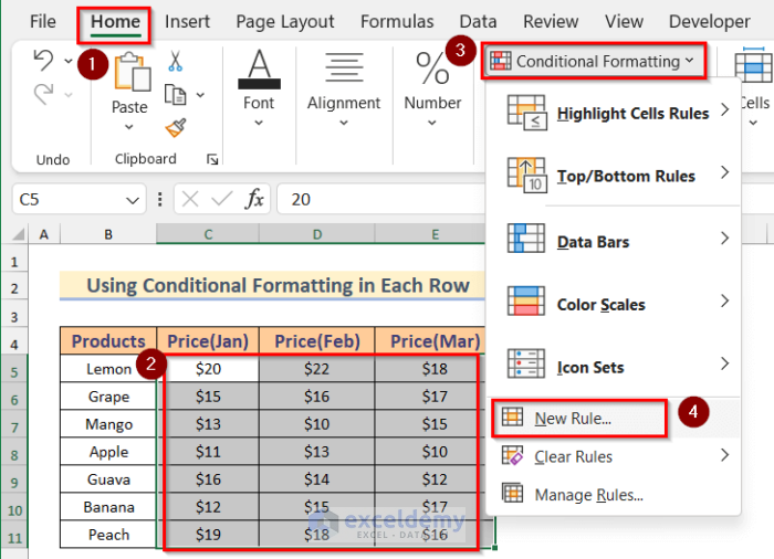
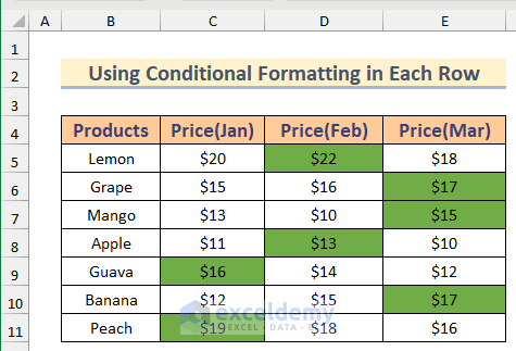
We’ll modify the dataset and use three columns to show prices for three consecutive months.

Steps:

• Select all three columns.
• Go to the Home tab, select Conditional Formatting, and choose New Rule.
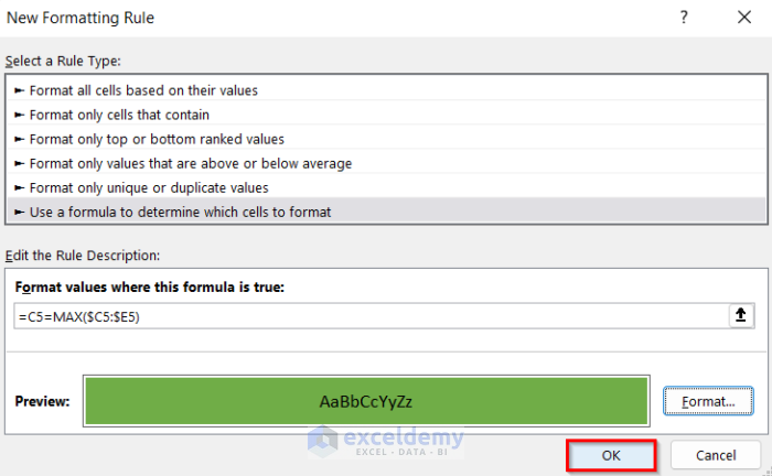
• A dialog box will appear.

• Choose Use a formula to determine which cells to format from the Select a Rule Type box.
• Copy the following formula in the Format values where this formula is true box.

• Press on the Format button. The Format Cells dialog box will open up.

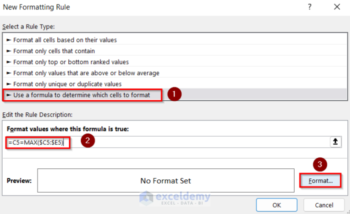
• Select your desired fill color and press OK. We have chosen the green color.

• Press OK again.

• The highest value of each row is highlighted with green.

Method 3 – Create an Excel Chart to Highlight the Highest Value in Excel

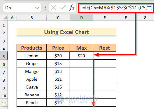
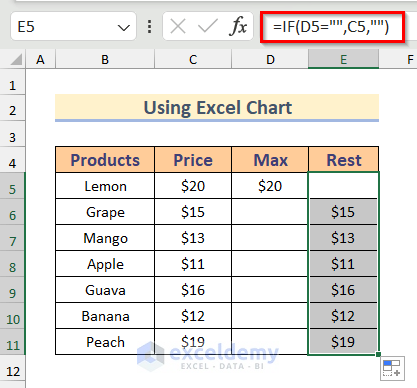
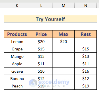
We have modified the sample dataset, adding two extra columns to represent the maximum value and the rest of the values.

Steps:

• Copy the following formula in Cell D5–

• Hit the Enter button and use the Fill Handle tool to copy the formula to the other cells.

• In Cell E5, insert the following formula:

• Press Enter and use the Fill Handle tool to copy the formula for the other cells.
• The maximum value and the rest of the values are separated into two columns.

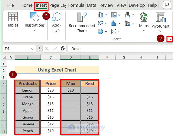
• Press and hold the Ctrl key and select the Products, Max, and Rest columns.
• Go to the Insert ribbon and click the arrow icon from the Charts bar.
• A dialog box named Insert Chart will appear.

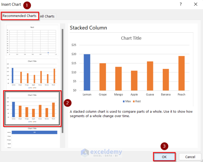
• Select the chart type you want from the Recommended Charts option and press OK.

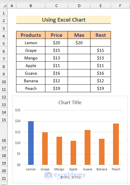
• The chart shows the highest value in a different color.

Read More: How to Highlight Text in Excel

Practice Section

You will find an Excel worksheet in the download file which you can use to practice on different datasets.

Download the Practice Book

Related Articles

• How to Highlight a Column in Excel
• How to Compare Two Excel Sheets and Highlight Differences
• How to Highlight Text in Text Box in Excel

<< Go Back to Highlight in Excel | Learn Excel