When you work on a large set of data, sometimes it is difficult to track where your cursor is and what kind of data you are looking for. To minimize this problem, you can use the highlighting option through which you can highlight a column in Excel. This process will automatically show you the highlighted columns. This article will provide a proper overview of how to highlight a column in Excel.
How to Highlight a Column in Excel: 3 Methods
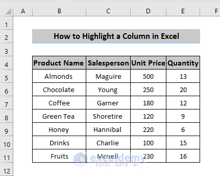
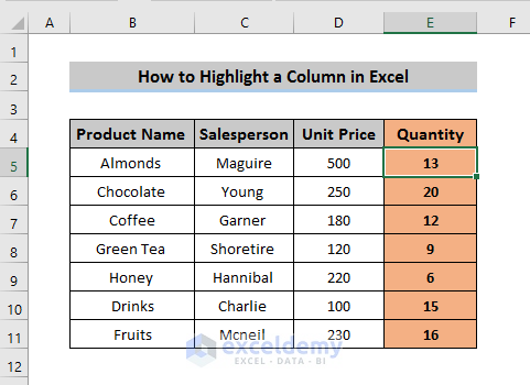
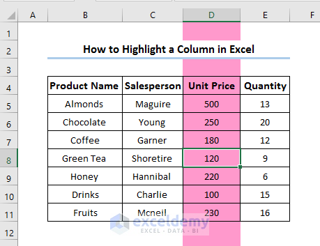
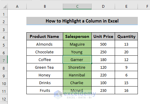
Here, we discuss three methods to highlight a column in Excel. All three methods are fairly easy to use and really effective in highlighting a column in Excel. To show all three methods we take a dataset that includes product name, Salesperson, unit price, and Quantity.
1. Highlight a Column Using Conditional Formatting
The first method is based on Conditional Formatting. This is a feature in which you can apply specific formatting for a certain criterion to selected cells. The conditional formatting method will change the overall appearance according to the given criteria. This method will give a fruitful solution to highlight a column in Excel.
Steps
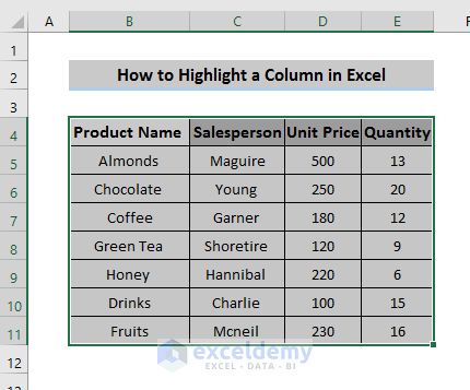
- To apply Conditional Formatting, first, select the cells where you want to apply this formatting.
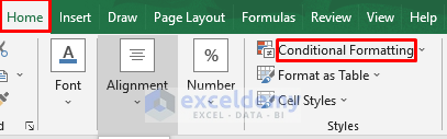
- Then, go to the Home tab in the ribbon, and in the Style section, you’ll get Conditional Formatting. Click on it.
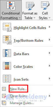
- In the Conditional Formatting option, select New Rule.
- After clicking the New Rule, a New Formatting Rule box will open up. In the ‘Select a Rule Type’ section, select ‘Use a formula to determine which cells to format’. A formula box will appear and write down the following formula in that box.
=CELL(“col”)=COLUMN()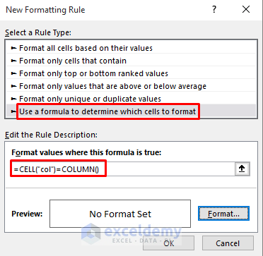
- Then select the Format option where you can format your column appearance after applying the rule. There is also a Preview section that shows your applied format preview.
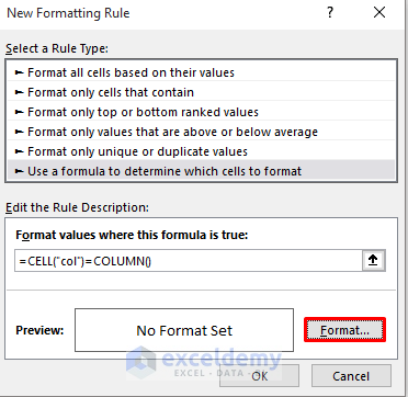
- In the Format option, you’ll get several options like font, border, and fill. Change appearance as your preference.
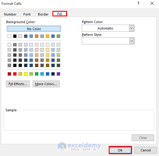
- After that click on ‘OK’
- Then, it shows that a column is highlighted but when you select the next column, nothing happens. By default, Excel doesn’t recalculate for selected changes, it only recalculates for editing the existing data or after entering new data. We need to press ‘F9’ for manual recalculation of the sheet. Press F9 first and then select the column you want to highlight. Then you’ll get the desired result.
- To eliminate this hassle, we have a great solution. First, open Visual Basic by pressing ‘Alt+F11’. Then go to the Microsoft Excel Object and select the sheet where you did this formatting.

- Copy the following code and paste it to the selected sheet and close the VBA Editor.
Private Sub Worksheet_SelectionChange(ByVal Target As Range)

    Target.Calculate

End Sub- There we have the required result. Now, you can select any column and it’ll automatically give the highlighted result. There is no need to press F9 anymore to recalculate.
Read More: How to Highlight from Top to Bottom in Excel
2. Using VBA Codes to Highlight a Column
Our next method is entirely based on the VBA codes. VBA codes make the process far easier than conditional formatting.
Steps
- To apply VBA codes, first, open the VBA Editor by pressing ‘Alt + F11’ or you can add the Developer tab by customizing the ribbon.
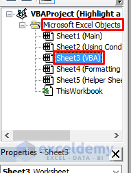
- Find the Microsoft Excel Object and select the preferred sheet where you want to apply the highlighting. As our sheet name is ‘VBA’, we select this sheet and double-click on it.
- A code window will appear copy the following code and paste it.
Private Sub Worksheet_SelectionChange(ByVal Target As Range)
    If Target.Cells.Count > 1 Then Exit Sub
    Application.ScreenUpdating = False

    'Clear the color of all cells
    Cells.Interior.ColorIndex = 0
       With Target
        'Highlight column of the selected cell
        .EntireColumn.Interior.ColorIndex = 38
    End With

    Application.ScreenUpdating = True
End Sub
Note: This code will clear the background color by setting ColorIndex to zero and it also highlights the column by setting ColorIndex to 38. You can apply any ColorIndex here
- Close the VBA Editor and there we have the required result.
Advantage
This method gives a better format than the previous method because here you don’t need to take the hassle of pressing F9 for recalculating. Only the VBA Code will give you the desired result.
Disadvantage
- This VBA code will clear all background colors so you can’t use any color when you apply this method.
- This code will block the undo function on this sheet
Read More: How to Highlight Text in Excel
3. Highlight a Column Using Conditional Formatting with VBA
When you use the previous two methods, you’ll find that the worksheet slows down gradually. To solve this problem, we can do the highlighting in such a way that we get the column number by VBA and use that number for the column function by conditional formatting formulas.
Steps
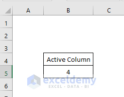
- First, add a new sheet to your workbook and name it ‘Assistant Sheet’. This sheet will store the number of columns. At a later point, the sheet can be hidden quite easily. We start from row 4 and column 2 because our main sheet starts this way. Then write the total no of columns where you want to apply this method.
- Then open the Visual Basic by pressing ‘Alt + F11’. Just like previous methods, go to the Microsoft Excel Object select the preferred sheet, and double-click on it. A code box will appear. Copy the following code and paste it
Private Sub Worksheet_SelectionChange(ByVal Target As Range)

    Application.ScreenUpdating = False

    Worksheets("Assistant Sheet").Cells(4, 2) = Target.Column

    Application.ScreenUpdating = True

End Sub- Now, to do the conditional formatting, select the dataset that you want to highlight.

- go to the conditional formatting from the Home tab in the ribbon and select the New Rule. From the New Rule option, select ‘use a formula to determine which cells to format’ just like the first method. There is a formula box where you need to apply the following formula
=COLUMN()=‘Assistant Sheet’!$B$4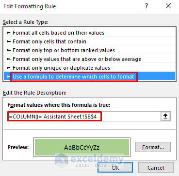
- You can change the appearance in your own style by using the Format that has been discussed in the first method. Then click on ‘OK’. There we have the desired result.
Download Practice Workbook
Download this practice workbook
Conclusion
Here, we have discussed three methods to highlight a column in Excel. I hope you find this very useful and easy to use. If you have any questions, feel free to comment below and let us know.
Related Articles
- How to Highlight Lowest Value in Excel
- How to Highlight Highest Value in Excel
- How to Compare Two Excel Sheets and Highlight Differences
- How to Highlight Text in Text Box in Excel
<< Go Back to Highlight in Excel | Learn Excel
Get FREE Advanced Excel Exercises with Solutions!
