In Microsoft Excel, we can highlight top to bottom values with the help of conditional formatting. Highlighting top and bottom values with different colors and shades is an easy process. In the following article, I am going to explain how to highlight top to bottom in Excel with conditional formatting and different formulas.
How to Highlight from Top to Bottom in Excel: 5 Quick Methods
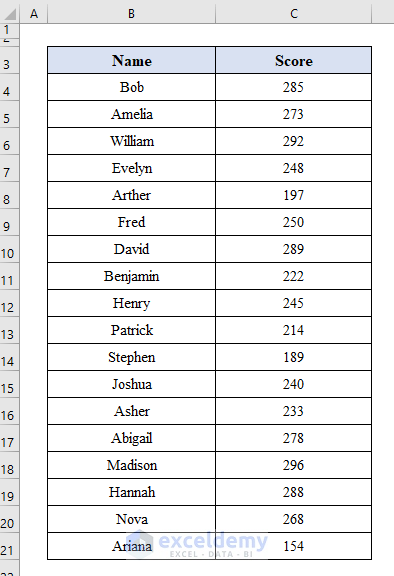
In the following section, we are explaining 5 quick methods to highlight from top to bottom. We took a dataset containing some names and their total scores. Now we will highlight from top to bottom with different methods.
1. Apply Conditional Formatting to Highlight from Top to Bottom in Excel
In this method, we will highlight top to bottom with conditional formatting.
Step 1:
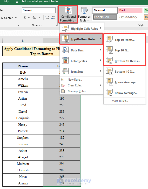
- Select Cells or Ranges to highlight.
- Under the Home ribbon, select the Top/Bottom Rules command from the Conditional Formatting
- Top/Bottom > Top 10 Items
Step 2:
- A Dialogue box named “Top 10 Items” will appear.
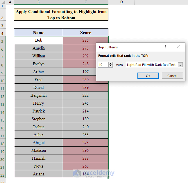
- Press OK.
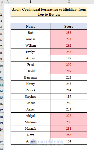
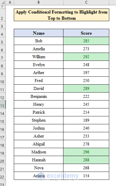
- Finally, the top 10 values in the dataset are highlighted.
Step 3:
Similarly, we can highlight the top 5 values from the dataset. The process is the same as in the previous discussion. But in the dialogue box “Top 10 Items”, we have to change the cell number to be highlighted. In the following picture, I have selected 5 cells with “Green Fill with Dark Green Text”.
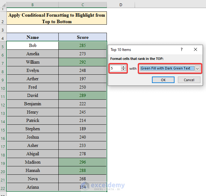
- After that, pressing OK we will find the top 5 values highlighted.
2. Perform a Custom Conditional Formatting Rule to Highlight from Top to Bottom
We will perform a custom conditional formatting rule to highlight from top to bottom in the following method.
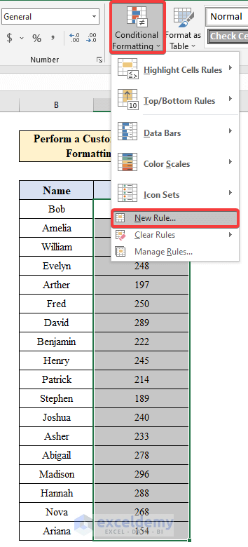
Step 1:
- Select the cells to highlight.
- Conditional Formatting > New Rule.
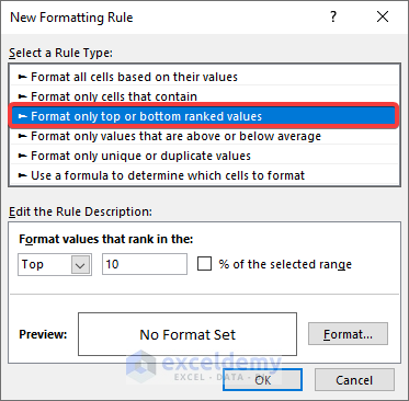
- A new dialogue box will appear named “New Formatting Rule”.
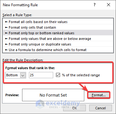
- Select “ Format only top or bottom ranked values” from the rule type.
Step 2:
- Select “Bottom”.
- Then type “25” and click on the “% of the selected range”. As we are highlighting the bottom 25% of values from the dataset.
- Press “Format”.
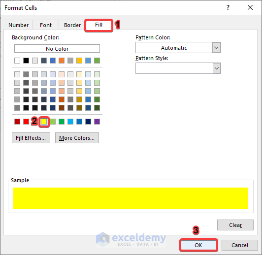
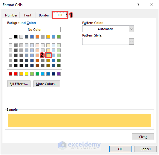
- A new dialogue box “Format Cells” will appear.
- Click on “Fill” and choose the desired color to highlight. I have selected yellow color to highlight.
Step 3:
- Press OK. A preview with yellow highlighted will appear.
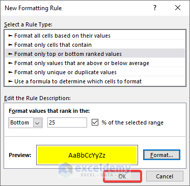
- Again press OK.
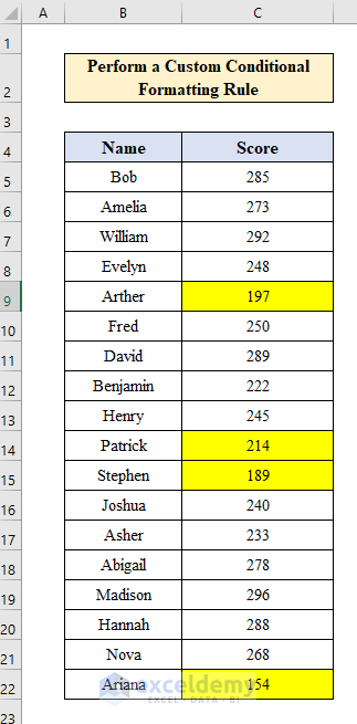
- Thus we will find our desired highlighted values from top to bottom.
Read More: How to Highlight Highest Value in Excel
3. Highlight N Values from Top to Bottom in Excel
Sometimes we have to highlight a selected number of values according to our requirements. In the following, we are going to describe how to highlight N’th values from top to bottom.
Step 1:
- Select Cells. Then navigate to:
Home > Conditional Formatting > Top/Bottom Rules > Bottom 10 Items.
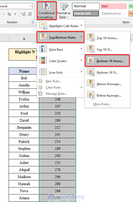
- A dialogue box “Bottom 10 Items”
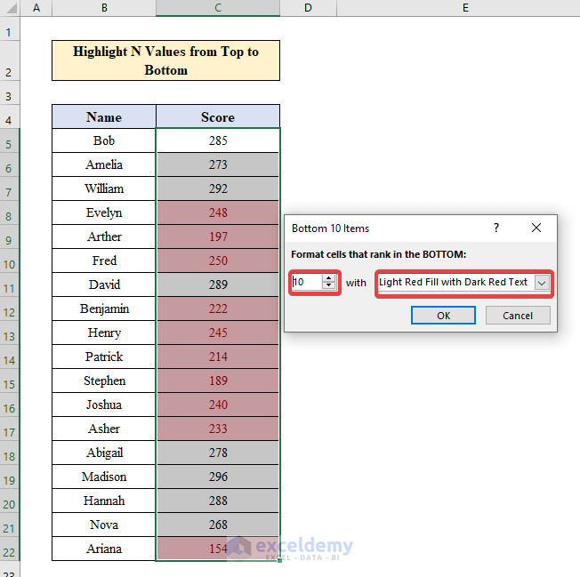
In the following, we can choose our desired N’th number of cells and change the highlight too.
Step 2:
- Choose “4” in the cell number.
- Change highlight to “Light Red Fill”.
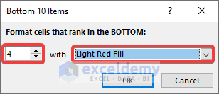
- Press OK.
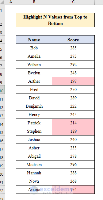
Here is our result with highlighted values from top to bottom.
Read More: How to Compare Two Excel Sheets and Highlight Differences
4. Use a Formula to Highlight from Top to Bottom in Excel
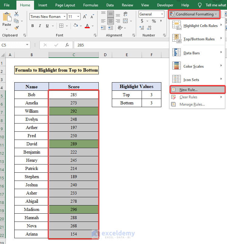
Now we will highlight top to bottom using formulas. In the dataset containing some names and scores. In the Highlight Values section, we have put “Top” and “Bottom”. The value we chose in both sections is “3” as we are going to show both the largest values from the top and the lowest values from the bottom.

Step 1:
- Select the range of cells in which the formula will be applied.
- Conditional Formatting > New Rule.
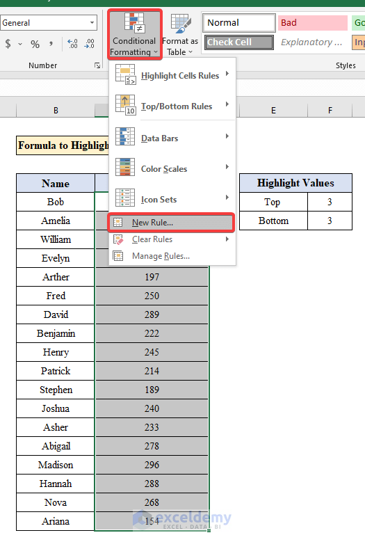
- A new dialogue box will appear “New Formatting Rule”.
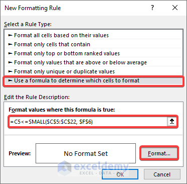
- Choose “Use a formula to determine which cells to format”.
Step 2:
- Apply the following formula-
=C5>=LARGE($C$5:$C$22, $F$5)Where,
- The LARGE Function is used to shade top numbers.
- ($C$5:$C$22)= It is the applied range.
- $F$5= It is used for the N values.
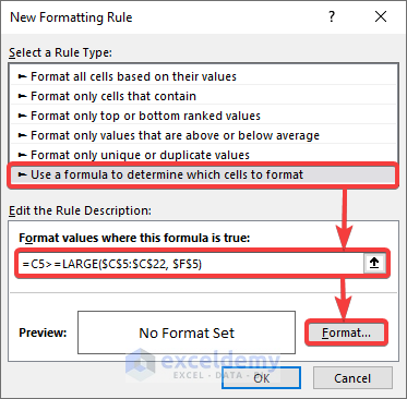
- Then click “Format”.
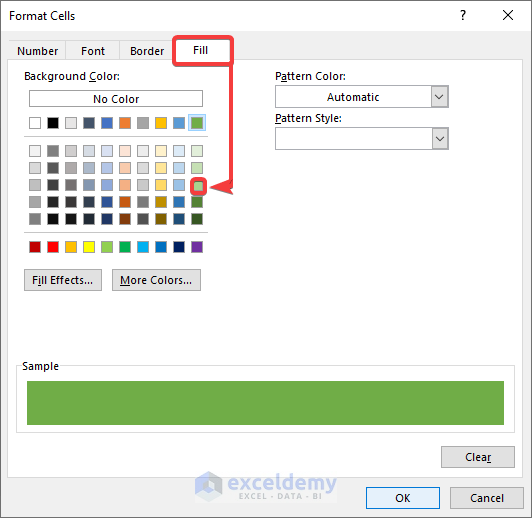
- Now click “Fill”.
- Then choose the color according to your choice. Here, I have chosen light green to highlight.
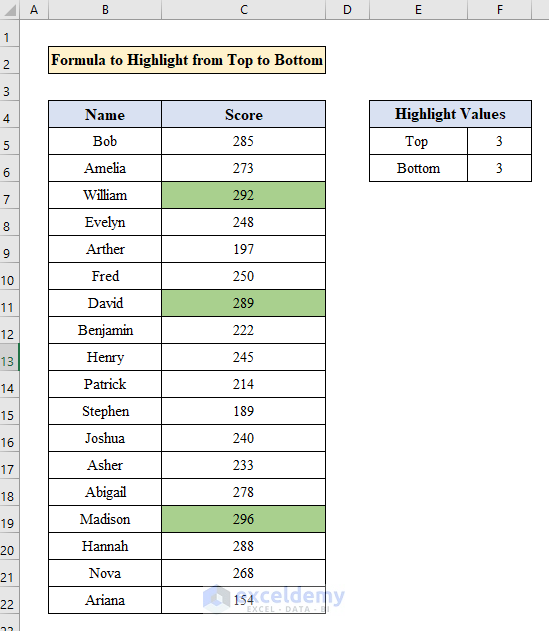
- So, we will find our top 3 largest values highlighted from the dataset.
Now, we will highlight the lowest values from the dataset.
Step 3:
- Select Cells.
- Conditional Formatting > New Rule.
- A new window will appear “New Formatting Rule”.
- Choose “Use a formula to determine which cells to format”.
Step 4:
- Apply the formula-
=C5<=SMALL($C$5:$C$22, $F$6)Where,
- The SMALL Function shades the bottom numbers.
- ($C$5:$C$22)= It is the range of cells.
- $F$6= It is N value.
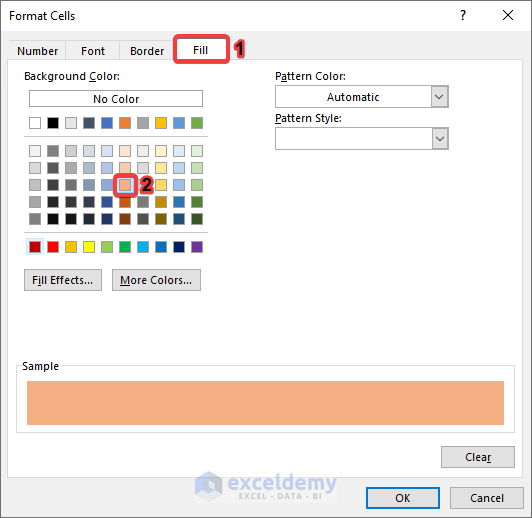
- Press Fill and choose the desired color.
- Now click OK.
- Here we got our lowest 3 values from our dataset.
Read More: How to Highlight Lowest Value in Excel
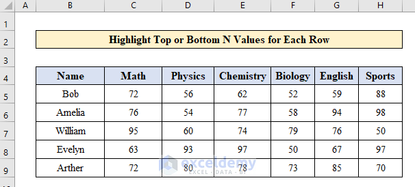
5. Apply a Formula to Highlight Top or Bottom N Values for Each Row in Excel
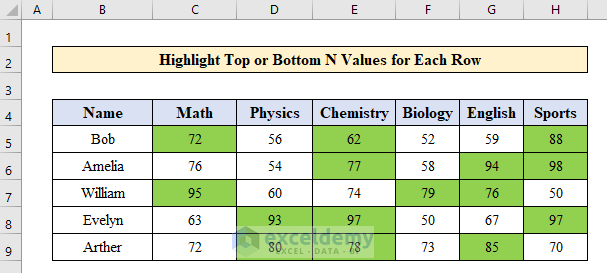
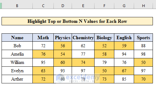
In this method, we will highlight the top or bottom n values for each row using a formula. The dataset contains some names and scores in different subjects. We will highlight the top three numbers in each row.
Step 1:
- Select all cells.
- Conditional Formatting > New Rule.
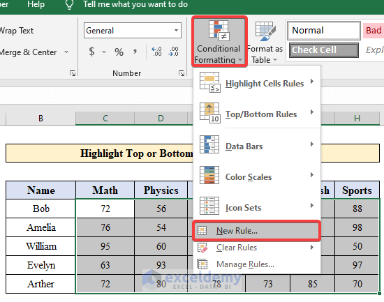
Step 2:
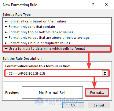
- A new dialogue box will appear “New Formatting Rule”.
- Select-” Use a formula to determine which cells to format”.
- Apply the formula-
=C5>=LARGE($C5:$H5,3)Where,
- The LARGE Function is used to shade top numbers.
- ($C5:$H5)= It is the range.
- “3” is used to show the top 3 numbers in each row.
- Click “Format”.
Step 3:
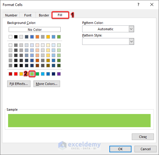
- A new window “Format Cells” will appear.
- Click “Fill” and select the desired color.
- Press OK.
- Here, the top 3 values in every row are highlighted.
Now we will highlight the lowest 3 values in each row. In the following, we will describe the method to do it.
Step 4:
- In the “Use a formula to determine which cells to format” box, apply this formula.
=C5<=SMALL($C5:$H5,3)Where,
- The SMALL Function shades the values.
- ($C5:$H5)= It is the range of data.
- “3” is used to select the lowest 3 values.
- Press “Format”.

Step 5:
- A new dialogue box will appear “Format Cells”.
- Choose “Fill” and the desired color.
- Press OK.
Here, we got the lowest 3 values highlighted in each row.
Read More: How to Highlight a Column in Excel
Things to Remember
- Select your range of cells before applying conditional formatting.
- Use the Absolute Cell References ($) to block cells otherwise, you won’t get the correct results.
Download Practice Workbook
Download this practice workbook to exercise while you are reading this article.
Conclusion
In this description, I have covered all the methods to highlight from top to bottom in Excel. If any problems, feel free to let us know in the comment section. Enjoy!
Related Articles
<< Go Back to Highlight in Excel | Learn Excel
Get FREE Advanced Excel Exercises with Solutions!
