Method 1 – Split Cells in Excel with the Text to Column Feature
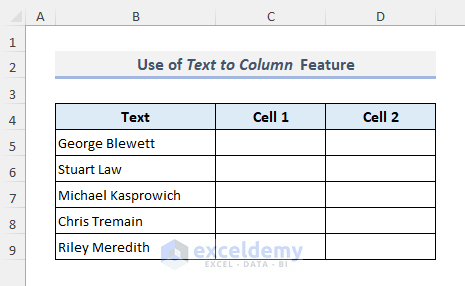
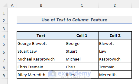
In the following table, we have some random names lying in the Text column. We’ll split each name into two parts. The first part will be displayed in Cell 1 column and another part in Cell 2 column.
Steps:
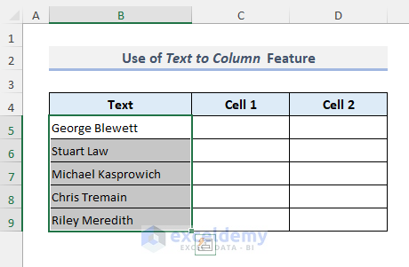
- Select the cells that you want to split into multiple cells.
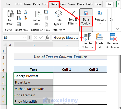
- From the Data tab, select the Text to Columns tool from the Data Tools group.
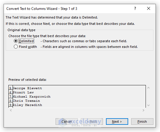
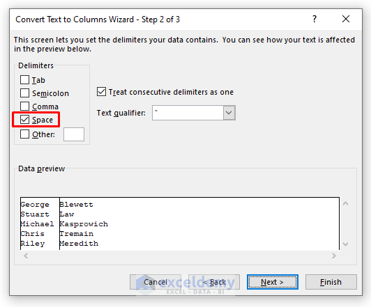
- In the wizard as shown below, click Next.
- From the Delimiters options, put a checkmark on Space only.
- Click Next.
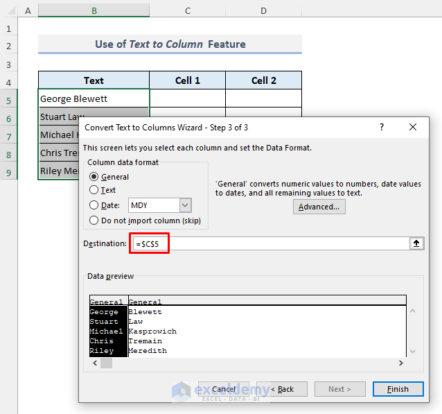
- Select the destination cell where you want to see the split cells.
- Press Finish.
- Here are the results.
Method 2 – Insert and Merge Columns to Split Cells in Excel
In the following table, we’ll divide the Name & Age column into two columns while keeping the header name unchanged.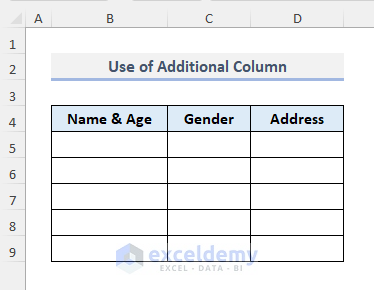
Steps:
- Select the Gender column.
- Right-click on it and choose the Insert option.
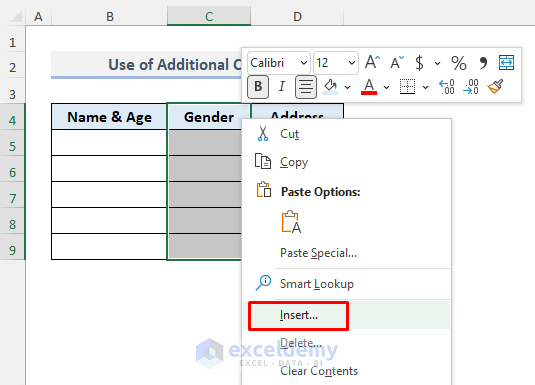
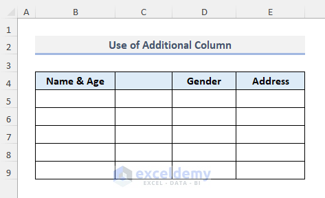
- An additional column has been added to the right of the Name & Age column.
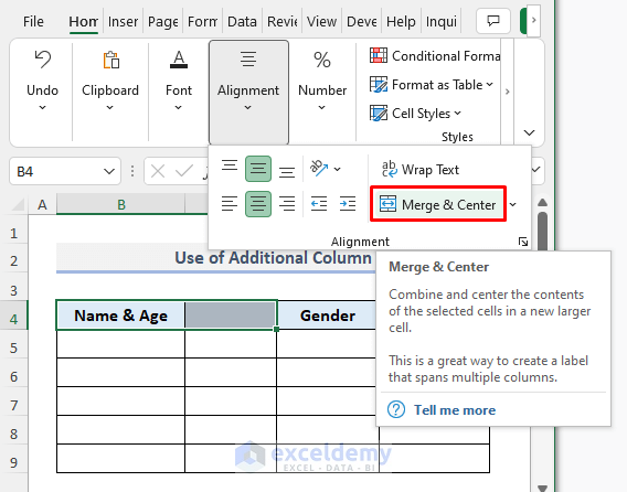
- Select the Name & Age header along with the blank header of the newly inserted column.
- From the Alignment group, click on the Merge & Center command.
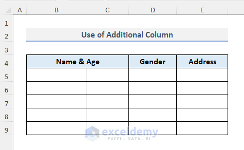
- The Name & Age column has been divided into two parts. You can also keep the headers separated by not choosing the option to merge them.
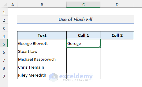
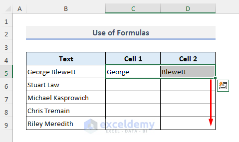
Method 3 – Apply Flash Fill to Divide Cells
Steps:
- Select cell C5 and type the first value you’re extracting from cell B5.
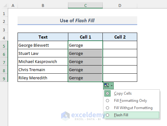
- Use the Fill Handle to autofill the entire column.
- From the AutoFill menu, choose the Flash Fill option.
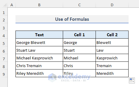
- The Cell 1 column is now showing all the first names from the Text column.
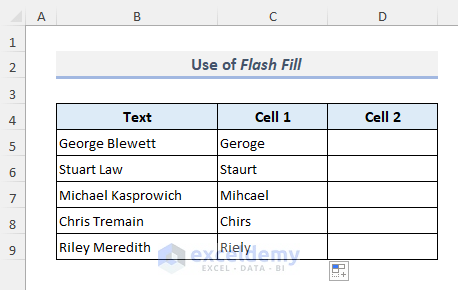
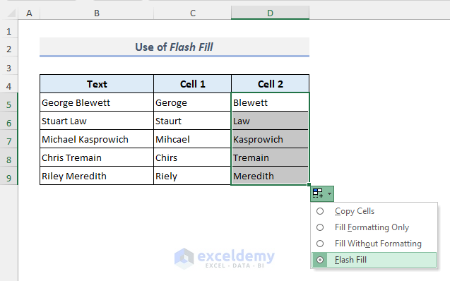
- Repeat for the second column.
Method 4 – Use Formulas to Split Cells in Excel
Case 4.1 – Combining LEFT and FIND Functions
Steps:
- Select cell C5 and insert the following formula.
=LEFT(B5,FIND(" ",B5)-1)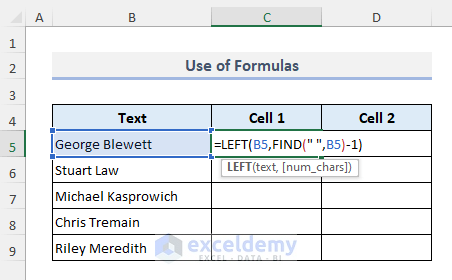
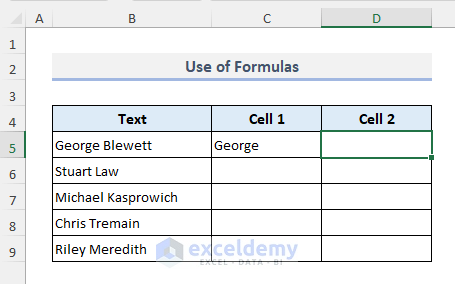
- Press Enter and you’ll get the first name of George Blewett.
How Does the Formula Work?
- FIND(” “,B5): The FIND function looks for the space character (“ “) in cell B5 and returns the position of that character which is 7.
- FIND(” “,B5)-1: After subtracting 1 from the previous result, the new return value here is 6.
- LEFT(B5,FIND(” “,B5)-1): Finally the LEFT function extracts the 1st 6 characters from the text in cell B5 which is George.
- Select cell D5 and use the following formula.
=RIGHT(B5,LEN(B5)-FIND(" ",B5))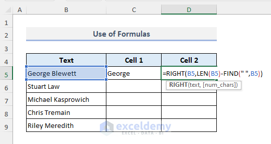
- Hit Enter.
How Does the Formula Work?
- LEN(B5): The LEN function counts the number of total characters found in cell B5 and thereby returns 14.
- FIND(” “,B5): The FIND function here again looks for the space character in cell B5 and returns the position which is 7.
- LEN(B5)-FIND(” “,B5): This part of the entire formula returns 7 which is the subtraction between the previous two outputs.
- RIGHT(B5,LEN(B5)-FIND(” “,B5)): Finally, the RIGHT function pulls out the last 7 characters from the text in cell B5 and that is Blewett.
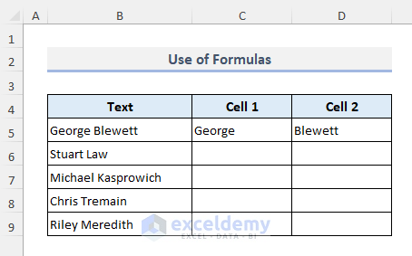
- Select both cells C5 and D5.
- Use the Fill Handle to drag down to the last output cell D9.
- Here’s the result.
Case 4.2 – Combining LEFT and SEARCH Functions
- Select cell C5 and then apply the following formula.
=LEFT(B5,SEARCH(" ",B5)-1)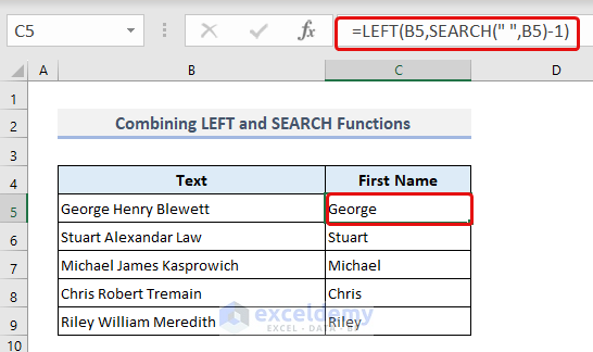
How Does the Formula Work?
- SEARCH(” “,B5): The SEARCH function looks for the space character (“ “) in cell B5 and returns the position of that character which is 7.
- SEARCH(” “,B5)-1: After subtracting 1 from the previous result, the new return value here is 6.
- LEFT(B5,SEARCH(” “,B5)-1): Finally the LEFT function extracts the 1st 6 characters from the text in cell B5 which is George.
Case 4.3 – Combining IFERROR, MID, and SEARCH Functions
We will get the middle name from the full name.
- Select cell C5 and paste the below formula.
=IFERROR(MID(B5,SEARCH(" ",B5)+1,SEARCH(" ",B5,SEARCH(" ",B5)+1)-SEARCH(" ",B5)),"")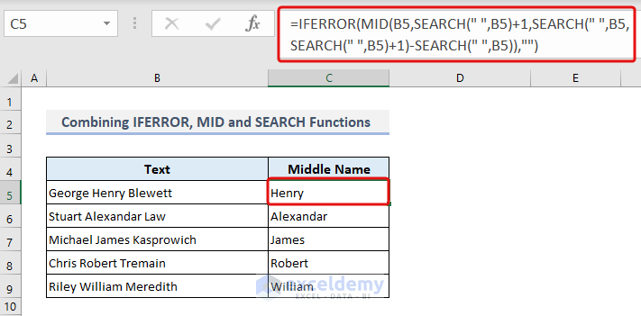
How Does the Formula Work?
- SEARCH(” “, B5): This portion searches for the position of the first space (” “) within the text in cell B5 and returns the position of that character which is 7.
- SEARCH(” “, B5, SEARCH(” “, B5)+1): This nested function searches for the position of the second space within the text in cell B5. It starts searching from the position immediately after the first space (found in step 1). It returns the numerical position of the second space character.
- MID(B5, SEARCH(” “, B5)+1, SEARCH(” “, B5, SEARCH(” “, B5)+1)-SEARCH(” “, B5)): This function extracts a substring from cell B5. It starts from the position immediately after the first space (found in step 1) and continues for a length determined by the difference between the positions of the first and second spaces (found in step 2). The MID function is used to perform this extraction.
- IFERROR(<substring extraction>, “”): The IFERROR function checks if there was an error during the substring extraction. If an error occurs (such as when the second space is not found), it returns an empty string (“”). If there is no error, it returns the extracted substring.
The formula checks if there is only one space in the text. If there is, it extracts the portion of the text after the first space. If there is more than one space, it extracts the portion after the second space.
Case 4.4 – Combining IF, LEN, SUBSTITUTE, RIGHT, and SEARCH Functions=
- Select cell C5 and enter the following formula.
=IF(LEN(B5)-LEN(SUBSTITUTE(B5," ",""))=1,RIGHT(B5,LEN(B5)-SEARCH(" ",B5)),RIGHT(B5,LEN(B5)-SEARCH(" ",B5,SEARCH(" ",B5)+1)))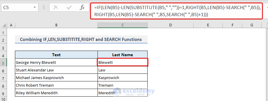
How Does the Formula Work?
Calculate the total length of the text in cell B5.
- LEN(B5): This function calculates the length of the text in cell B5.
Count the number of spaces in the text.
- SUBSTITUTE(B5,” “,””): The SUBSTITUTE function replaces spaces with an empty string (i.e., removes spaces) in the value of cell B5.
- LEN(B5)-LEN(SUBSTITUTE(B5,” “,””)): This subtraction gives the count of spaces in the text.
Check if there is only one space.
- LEN(B5)-LEN(SUBSTITUTE(B5,” “,””))=1: This comparison checks if the count of spaces is equal to 1.
Extract the desired portion of the text based on the number of spaces.
If there is only one space (True condition):
- SEARCH(” “,B5): This function finds the position of the first space in the text.
- LEN(B5)-SEARCH(” “,B5): This subtraction calculates the number of characters from the first space to the end of the text.
- RIGHT(B5,LEN(B5)-SEARCH(” “,B5)): This function extracts the right portion of the text starting from the position after the first space.
If there are multiple spaces (False condition):
- SEARCH(” “,B5,SEARCH(” “,B5)+1): This nested SEARCH function finds the position of the second space in the text.
- LEN(B5)-SEARCH(” “,B5,SEARCH(” “,B5)+1): This subtraction calculates the number of characters from the second space to the end of the text.
- RIGHT(B5,LEN(B5)-SEARCH(” “,B5,SEARCH(” “,B5)+1)): This function extracts the right portion of the text starting from the position after the second space.
Combine the true and false conditions using the IF statement.
- IF(LEN(B5)-LEN(SUBSTITUTE(B5,” “,””))=1, RIGHT(B5,LEN(B5)-SEARCH(” “,B5)), RIGHT(B5,LEN(B5)-SEARCH(” “,B5,SEARCH(” “,B5)+1))): This IF statement checks if there is only one space in the text. If true, it extracts the portion after the first space; otherwise, it extracts the portion after the second space.
In summary, this formula checks the number of spaces in the text. If there is only one space, it extracts the portion of the text after the first space. If there are multiple spaces, it extracts the portion after the second space.
Method 5 – Split Cells Using Excel Power Query
Steps:
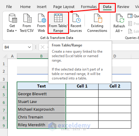
- Select the surnames from the entire column including the header.
- Go to the Data tab and choose the option From Table/Range in the Get & Transform Data group.
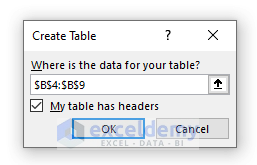
- In the Create Table dialog box, check the My table has headers option.
- Press OK.
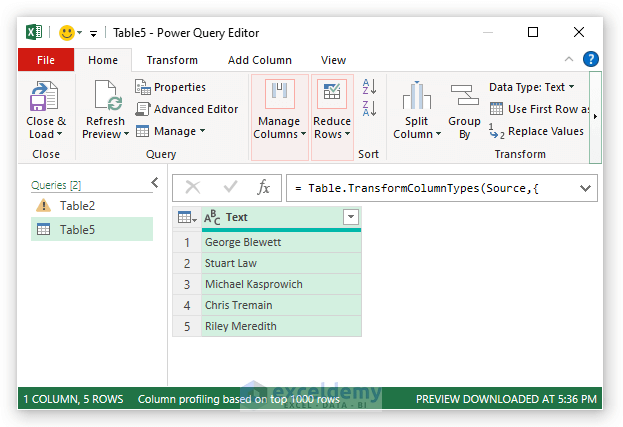
- The Power Query Editor will open up, where we’ll find our selected data as displayed below.
- Hover over the header Text.
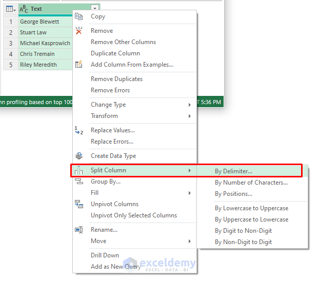
- Open the Context Menu by right-clicking.
- From the Split Column menu, select the option By Delimiter.
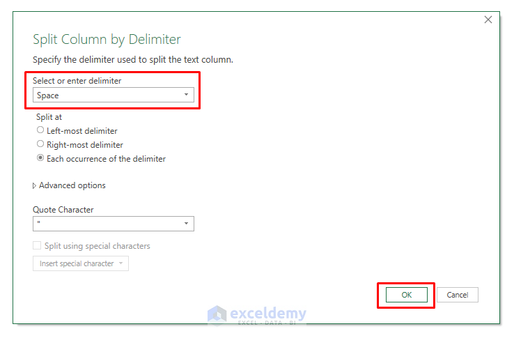
- Specify the delimiter Space as shown inside the highlighted border since the texts in our dataset are delimited by spaces.
- Press OK.
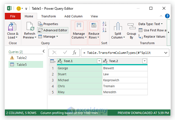
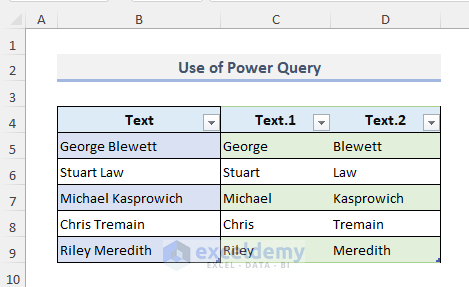
- In the Power Query window, you’ll find the selected texts in two parts.
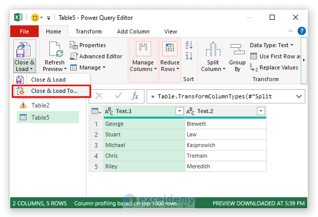
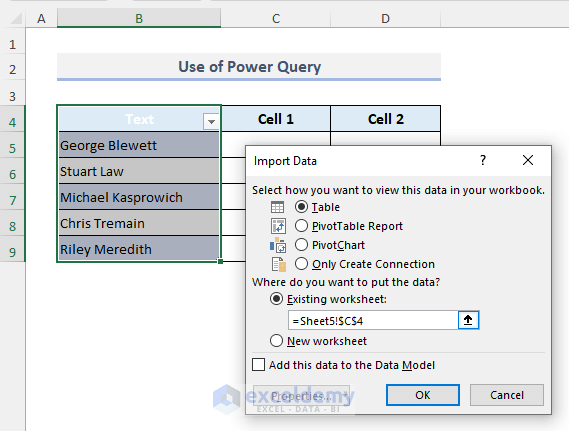
- From the Close & Load drop-down, choose the option Close & Load to…
- Select the output cell from where the split texts along with their headers will be displayed.
- Press OK.
- The following table is the final output.
Method 6 – Split Cells Into Rows in Excel
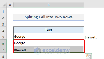
Case 6.1 – Split Cells into Two Rows
We took a random name and split that name into the 6th and 7th rows.
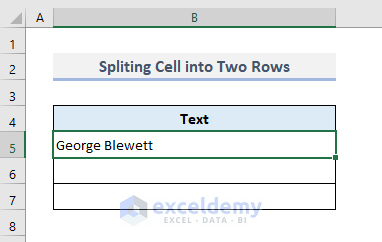
- Use the Text to Column feature to split the cell value into two columns. We have discussed this in this article earlier.
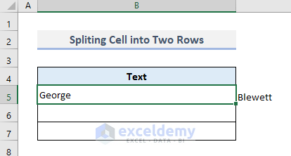
- Select cells B5 and C5. Press Ctrl + C to copy the cells.
- Select cell B6 and paste them with Paste Special, then choose Transpose.
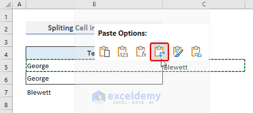
- Here’s the result.
Case 6.2 – Split Cells into Multiple Rows
- Select cell B6 and enter the following formula.
=FILTERXML("<t><s>" &SUBSTITUTE(B5," ", "</s><s>") & "</s></t>", "//s")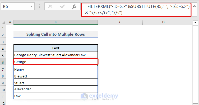
How Does the Formula Work?
- “<t><s>” &SUBSTITUTE(B5,” “, “</s><s>”) & “</s></t>”: This concatenates the opening <t><s> and closing </s></t> tags to the text in cell B5. It also replaces each space in the text with </s><s> to create separate <s> elements for each word.
- FILTERXML(xml, xpath): This function parses XML content and extracts specific elements based on an XPath expression.
- xml: The XML content to parse. In this case, it’s the string generated in step 1, which contains a series of <s> elements representing each word.
- xpath: The XPath expression that specifies the elements to extract. In this case, “//s” is used, which selects all <s> elements.
- “//s”: This XPath expression selects all <s> elements from the XML content.
The formula takes the text in B5, and converts it into an XML string where each word is represented by a separate <s> element, and then extracts all the words using the FILTERXML function with the XPath expression //s. This allows you to split the text into individual words.
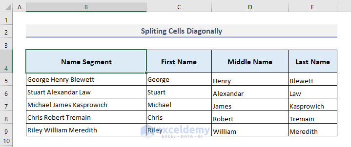
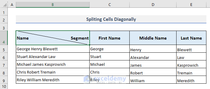
How to Split Cells Diagonally in Excel
We will split cell B4 diagonally.
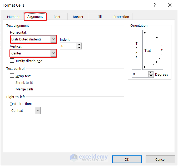
- Select cell B4 and then press Ctrl + 1. A pop-up window of Format Cells will appear.
- Go to the Alignment section and, in the Text alignment area, change the following:
Horizontal: >> Distributed (Indent)
Vertical: >> Center
- Go to the Border section.
- Select the diagonal outline like the image below and change the color to Black.
- Press OK.
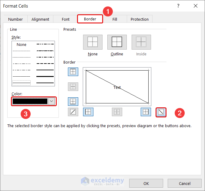
- The cell has been diagonally split.
How to Split a Merged Cell into Multiple Cells
We took some names in merged cells.
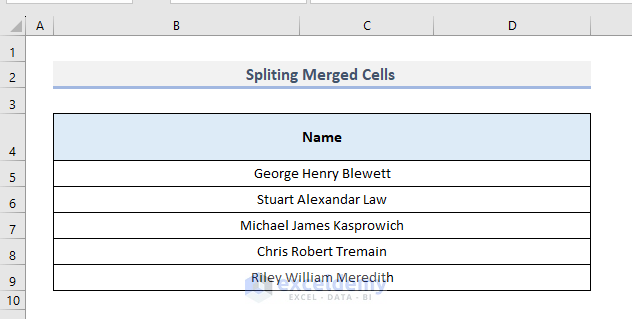
- Select the merged cell B5 and go to the Home tab.
- From the Alignment section, select Merge & Center drop-down and select Unmerge Cells.
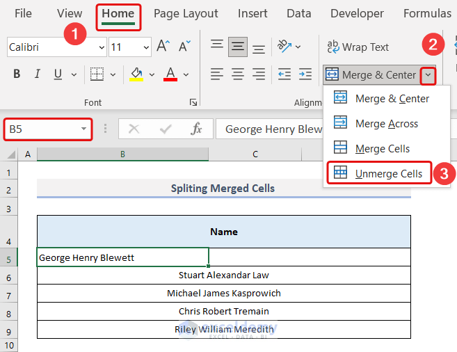
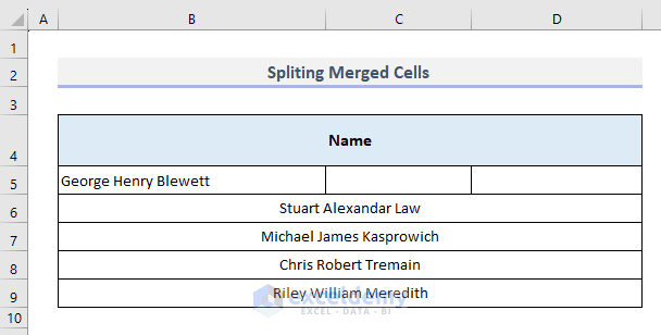
- You’ll find the cell has been split.
Things to Remember
- Backup your data: Before splitting cells, it’s always a good practice to create a backup of your data or work with a copy of the original data. This ensures that you have a safe copy in case any issues arise during the splitting process.
- Select the correct delimiter: When using methods like Text to Columns, you’ll need to specify the delimiter that separates the content you want to split. Common delimiters include commas, spaces, tabs, semicolons, or custom characters. Ensure that you select the correct delimiter that matches your data.
- Choose the right destination: Decide whether you want to split the cell contents into multiple columns or rows. In the case of Text to Columns, you can choose to split the data directly into adjacent columns or overwrite the existing data.
Frequently Asked Questions
Can you split a text box?
Yes, you can split a text box. Fill out a single textbox with text, then select it and click Split Join. Based on the carriage returns in the text, the text will be divided into several text boxes. When copying text from Word or another document, this feature is really useful.
How to extract data in Excel?
Manual extraction is the simplest extraction method. To use it, you need to open your dataset and select the data you want to extract. Then, copy the selected data and paste it into a new spreadsheet or another app where you need to work with that information.
Can I undo cell splitting in Excel?
Unfortunately, Excel does not have a built-in undo feature specifically for cell splitting. However, you can manually revert the changes by undoing or reentering the split data. It’s always recommended to back up your data before splitting cells to avoid accidental changes.
Can I split cells based on custom delimiters?
Yes, you can split cells based on custom delimiters in Excel. In the Text to Columns Wizard, choose the option Delimited and enter your custom delimiter in the provided field.
Download the Practice Workbook
Get FREE Advanced Excel Exercises with Solutions!
