How to Extract Specific Numbers from a Cell in Excel (11 Ways)

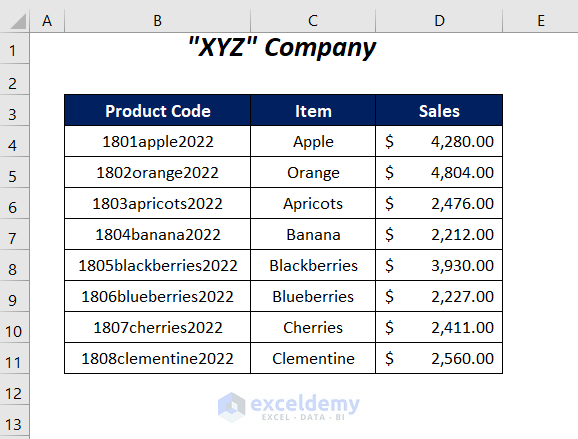
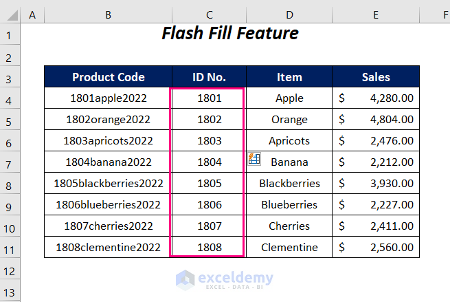
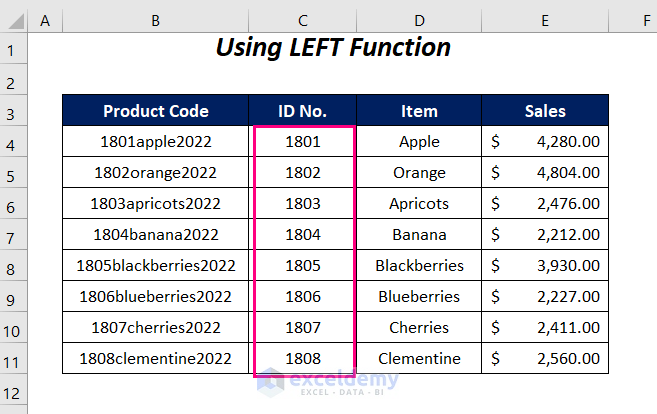
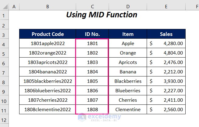
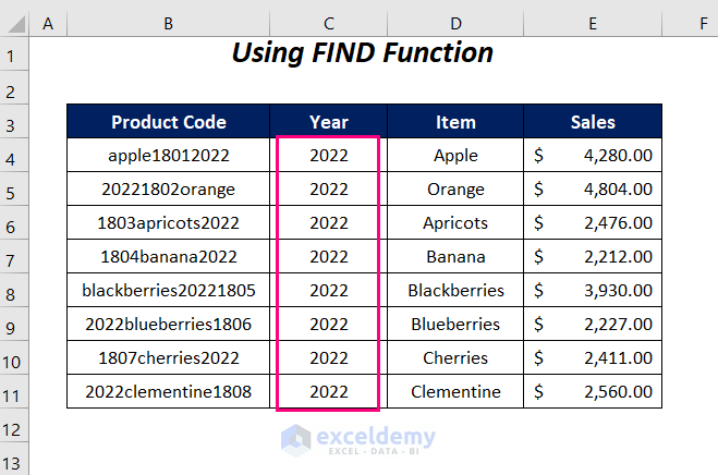
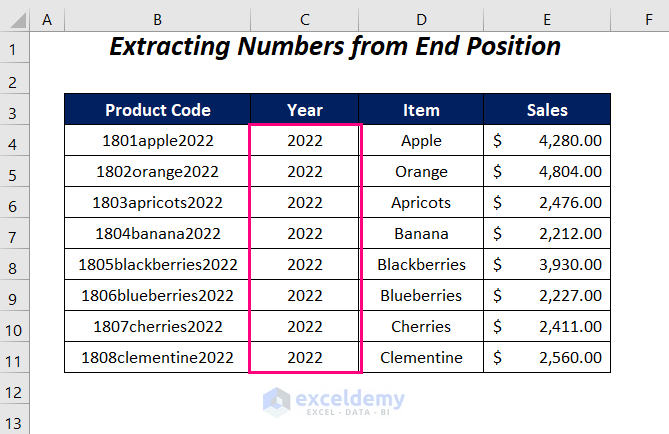
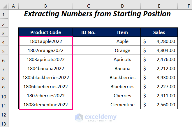
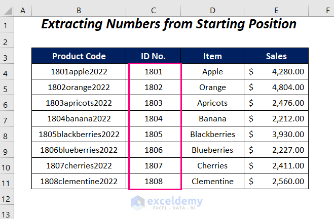
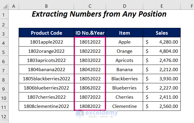
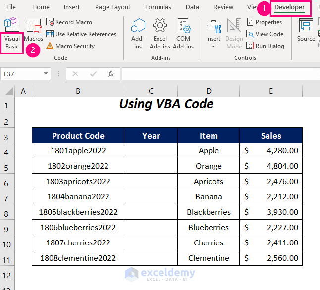
Consider the following dataset containing the product codes and sales records of some items. The product codes are created with a combination of the items’ id numbers, their name, and respective years. We will show how to extract the specific numbers from these codes.

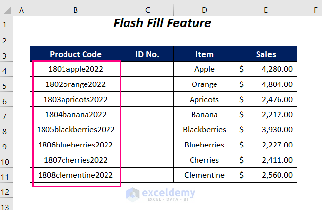
Method 1 – Using Flash Fill Feature to Extract Specific Numbers from an Excel Cell

The Flash Fill feature can extract a single number sequence if it follows a pattern throughout the column. Let’s use it for the ID Number at the front.

Steps:

• Manually write part of the ID Numbers from the B column in the first two cells, C4 and C5.

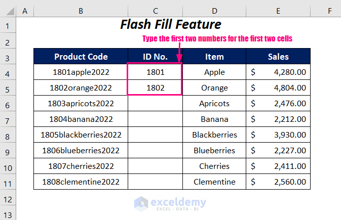
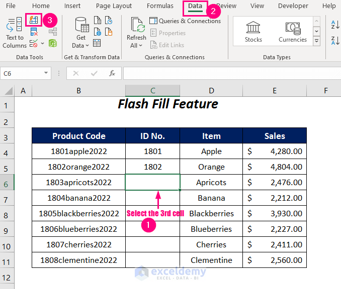
• Select the third cell, C6.
• Go to the Data Tab, Data Tools Group, and select the Flash Fill option.

• The ID No. column should be filled out with the ID Numbers from the Product Codes.

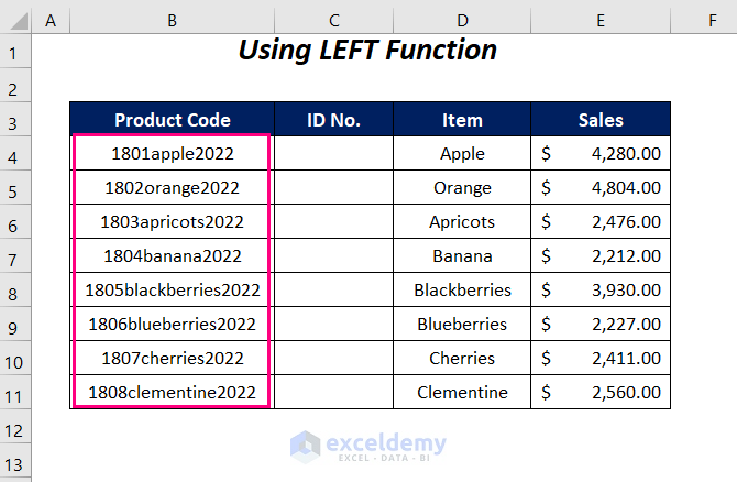
Method 2 – Using Excel LEFT Function to Extract Specific Numbers

Here, we will use the LEFT function to extract the ID Numbers from the Product Codes and the VALUE function to convert the extracted strings into numeric values.

Steps:

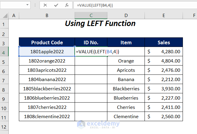
• Type the following function in cell C4:

Here, B4 is the Product Code, and 4 is for extracting the first four characters from the left. As LEFT will extract the specific numbers as text strings, VALUE will convert the extracted strings into numeric values.

• Press Enter and drag down the Fill Handle tool.

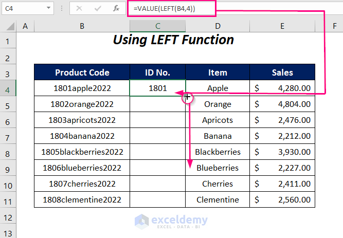
• You will get the ID Numbers of the products in the ID No. column.

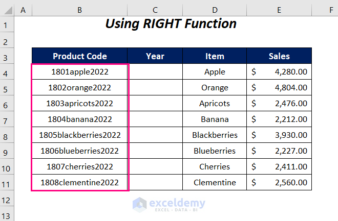
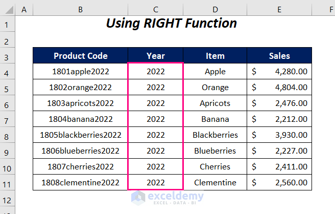
Method 3 – Inserting Excel RIGHT Function to Extract Specific Numbers

Let’s use the RIGHT function to extract the Years values into the Year column.

Steps:

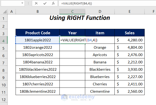
• Type the following function in cell C4:

B4 is the Product Code, and 4 is for extracting the last four characters from the right. RIGHT will bring out the specific numbers as text strings, and VALUE will convert those strings into numeric values.

• Press Enter and drag down the Fill Handle tool.

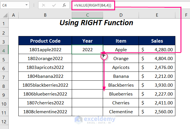
• We get the years from the Product Codes in the Year column.

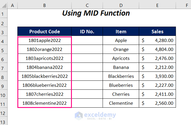
Method 4 – Using Excel MID Function to Extract Specific Numbers from a Cell

Let’s use the MID function to extract the first four numbers of the Product Codes into the ID No. column.

Steps:

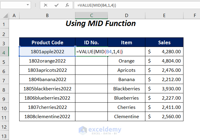
• Type the following function in cell C4:

Here, B4 is the Product Code, 1 is the starting number, and 4 is for extracting the first four characters from the start position. While MID will extract the specific numbers as text strings, VALUE will convert the extracted strings into numeric values.

• Press Enter and drag down the Fill Handle tool.

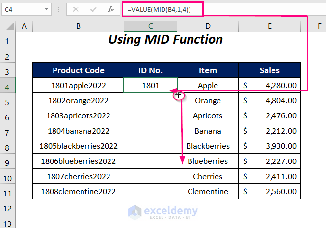
• The ID No. column will populate.

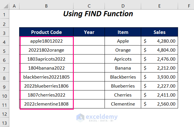
Method 5 – Obtaining Specific Numbers from Any Position with Excel FIND Function

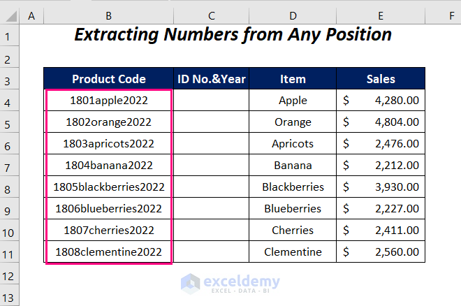
For this section, we have rearranged the Product Codes randomly to extract the years from any position of these codes with the help of the MID function and FIND function.

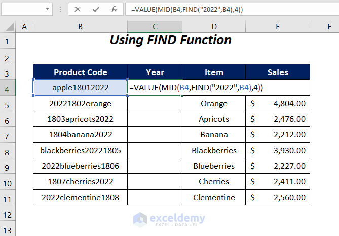
Steps:

• Type the following function in cell C4:

• Press Enter and drag down the Fill Handle tool.

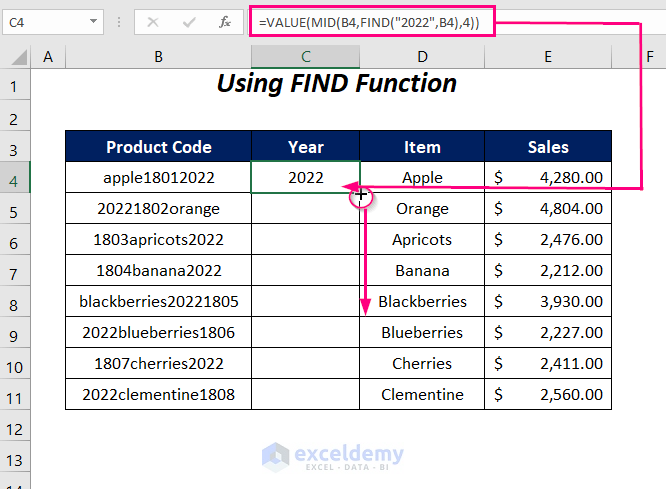
• We will have the years from the Product Codes in the Year column.

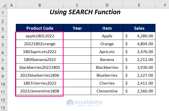
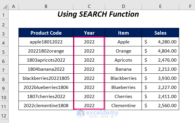
Method 6 – Extracting Specific Numbers from Any Position of a Cell Using SEARCH Function

Like the previous method here we will also search for the specific numbers 2022 in the randomly created Product Codes.

Steps:

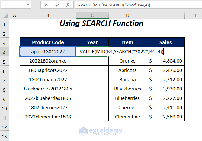
• Type the following function in cell C4.

• Press Enter and drag down the Fill Handle tool.

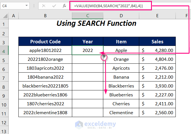
• The Year column will be filled.

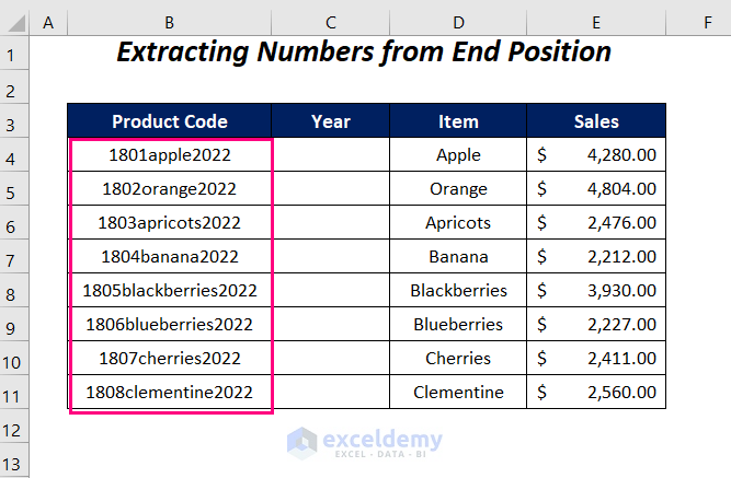
Method 7 – Extracting Specific Numbers from the End Position of Cells in Excel

We will extract all of the numbers after the text values in the Product Codes with the combination of the IFERROR, VALUE, RIGHT, LEN, MAX, IF, ISNUMBER, MID, ROW, INDIRECT functions.

Steps:

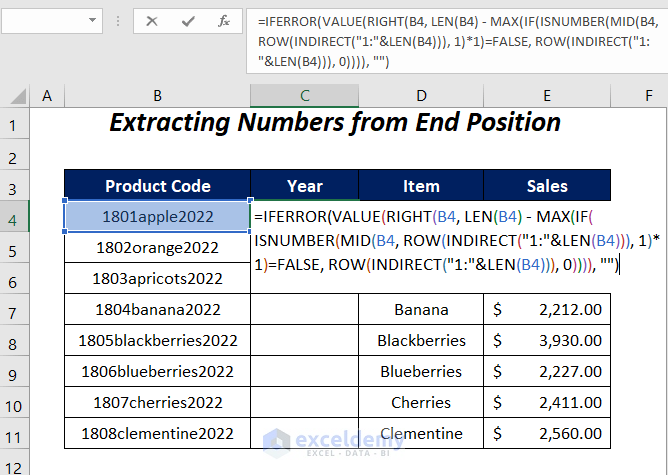
• Type the following function in cell C4:

• Press Enter (or Ctrl + Shift + Enter if the function doesn’t work) and drag down the Fill Handle tool.

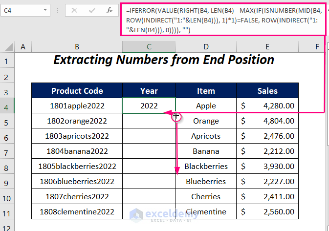
• You will get the specific numbers from the end of the cell and can extract any number of values by using this formula.

Method 8 – Extracting Specific Numbers from Starting Position of Cells

Similarly, we can extract all of the numbers before the text values in the Product Codes with the combination of the IFERROR, VALUE, LEFT, LEN, MATCH, IF, ISNUMBER, MID, ROW, INDIRECT functions.

Steps:

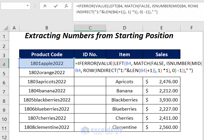
• Type the following function in cell C4.

• Press Enter and drag down the Fill Handle tool.

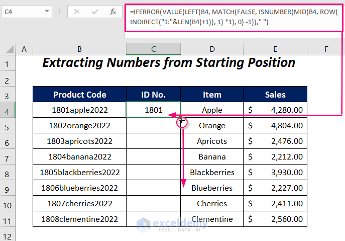
• You will get the specific numbers at the start of the cell and can extract any number of values by using this formula.

For offline versions of Excel, press Ctrl + Shift + Enter instead of pressing Enter.

Method 9 – Getting All Numbers from Any Position of Cells in Excel

Here, we will gather all of the numeric values which means the ID numbers and the years together in the ID No.&Year column with the help of the SUMPRODUCT, MID, LARGE, INDEX, ISNUMBER, ROW, INDIRECT, LEN functions.

Steps:

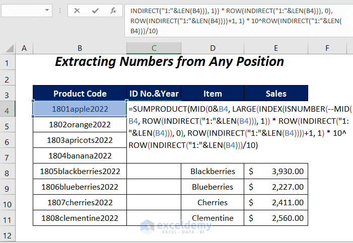
• Type the following function in cell C4.

• Press Enter and drag down the Fill Handle tool.

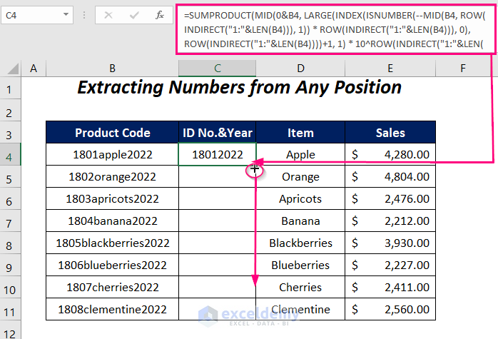
• We will get the concatenation of our specified numbers.

When using other Excel versions except Microsoft Excel 365, press Ctrl + Shift + Enter instead of Enter.

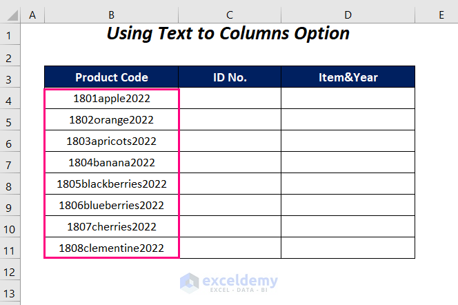
Method 10 – Using Excel’s Convert Text to Columns Wizard to Get Specific Numbers

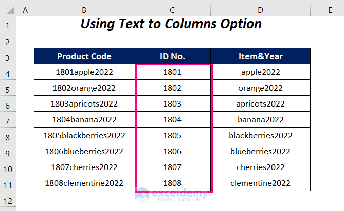
Let’s separate the decimal numbers from the product codes in the ID No. column.

Steps:

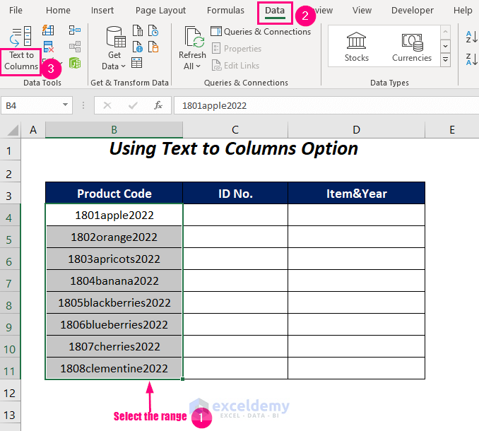
• Select the range.
• Go to the Data tab, Data Tools group, and choose the Text to Columns option.

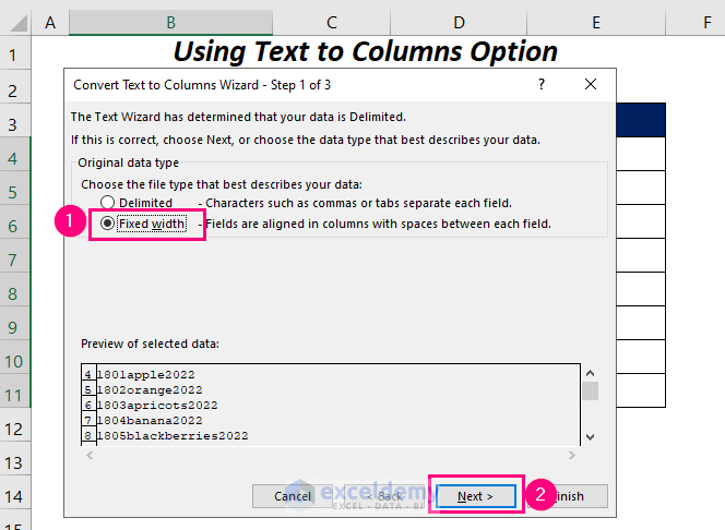
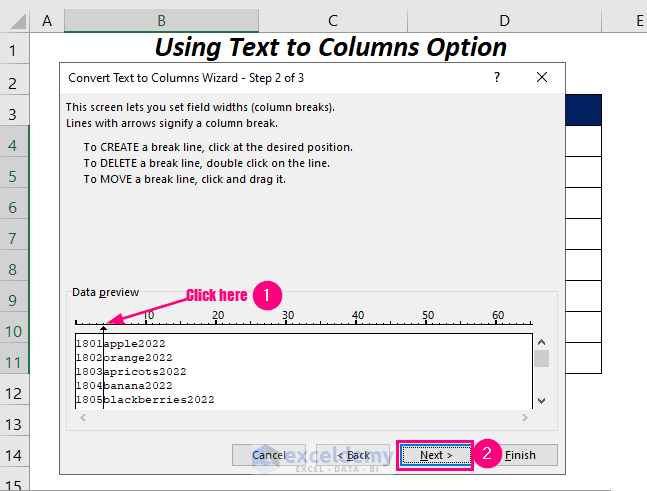
• The Convert Text to Columns Wizard will appear.
• Click on the Fixed width option and press Next in the first step.

• Click on the position where you want the separation (as we want to have the division after the ID Numbers, we have clicked after it)
• Press Next.

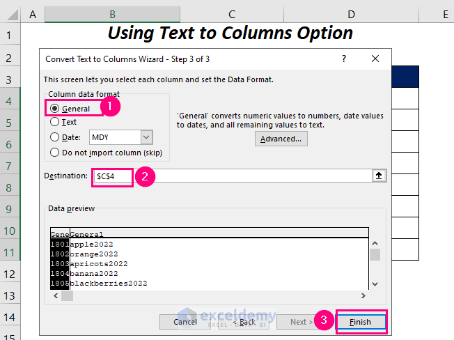
• In Column data format, select General.
• For Destination, put $C$4.
• Press Finish.

• We should have our desired ID Numbers in the ID No. column.

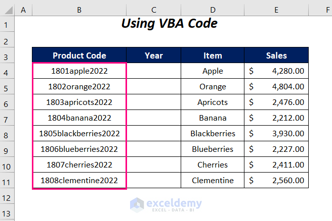
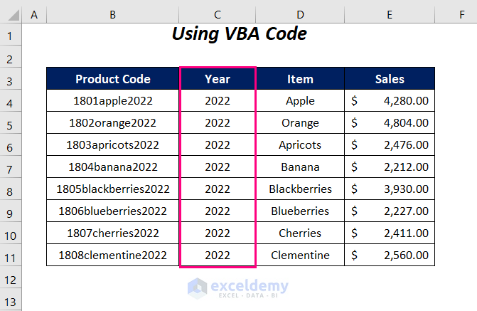
Method 11 – Using VBA Macro to Extract Specific Numbers from a Cell

In this section, we are going to use a VBA code to remove numbers from the string.

Steps:

• Go to the Developer tab and select Visual Basic.

• The Visual Basic Editor will open up.
• Go to the Insert Tab and choose Module.

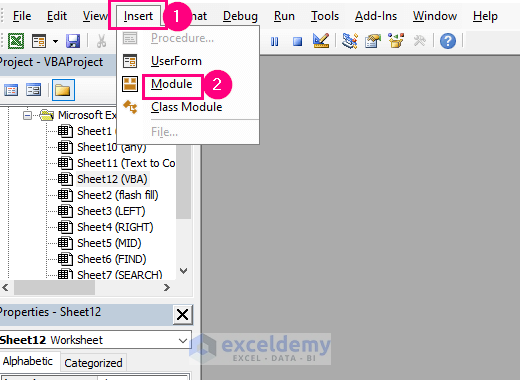
• After that, a Module will be created.

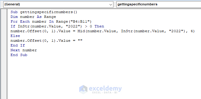
• Copy the following code:

Sub gettingspecificnumbers()
Dim number As Range
For Each number In Range("B4:B11")
If InStr(number.Value, "2022") > 0 Then
number.Offset(0, 1).Value = Mid(number.Value, InStr(number.Value, "2022"), 4)
Else
number.Offset(0, 1).Value = ""
End If
Next number
End Sub

Here, we have declared the number as Range, and it will store each value of the cells for the range B4:B11 within the FOR loop. IF statement will check whether the values contain a specific portion of 2022 with the help of the InStr function which looks for a partial match.
For matching the criteria, we will extract the portion 2022 from the strings in the adjacent cells.

• Press F5.
• In this way, you will get the years in the Year column after the extraction from the codes.

Download Practice Workbook

<< Go Back to Separate Numbers Text | Split | Learn Excel