Method 1 – Separate Numbers after a Particular Text with Excel Functions
1.1 Insert TEXTJOIN, IFERROR, MID, ROW, INDIRECT & LEN Functions
STEPS:
- Select cell C5.
- Copy the following formula in that cell:
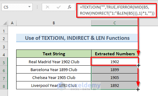
=TEXTJOIN("",TRUE,IFERROR(MID(B5,ROW(INDIRECT("1:"&LEN(B5))),1)*1,""))- Press Enter.
- In cell C5 the above command returns the number part from the string of cell B5.
- Drag the fill handle tool from cell C5 to C8 to autofill the remaining dataset.
- Get the result like the following image.
How Does the Formula Work?
- INDIRECT(“1:”&LEN(B5)): The INDIRECT function takes the value of LEN(B5) as cell reference which is 26.
- ROW(INDIRECT(“1:”&LEN(B5))): The Row function uses the return value by the INDIRECT function as a reference.
- MID(B5,ROW(INDIRECT(“1:”&LEN(B5))),1): The MID function extracts the number of parts from cell B5.
- IFERROR(MID(B5,ROW(INDIRECT(“1:”&LEN(B5))),1)*1,””): If the MID function finds a valid value the IFERROR function returns that otherwise it returns blank.
- TEXTJOIN(“”,TRUE,IFERROR(MID(B5,ROW(INDIRECT(“1:”&LEN(B5))),1)*1,””)): The TEXTJOIN function returns the number part from the string in cell B5.
1.2 Combine LOOKUP, MID, MIN & FIND Functions
STEPS:
- Select cell C5.
- Type the below formula in that cell:
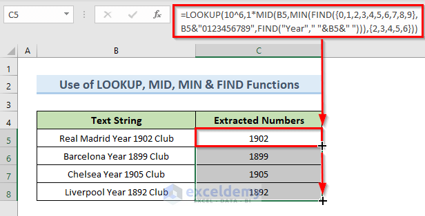
=LOOKUP(10^6,1*MID(B5,MIN(FIND({0,1,2,3,4,5,6,7,8,9},B5&"0123456789",FIND("Year"," "&B5&" "))),{2,3,4,5,6}))- Press Enter.
- It returns the number part in cell C5 from the string of cell B5 after the text Year.
- Drag the Fill Handle tool from cell C5 to C8 to autofill the dataset.
- Get results like the image below.
How Does the Formula Work?
- FIND(“Year”,” “&B5&” “): The text value Year in cell B5.
- FIND({0,1,2,3,4,5,6,7,8,9},B5&”0123456789″,FIND(“Year”,” “&B5&” “)): This part finds the numeric values after the text Year in cell B5.
- MIN(FIND({0,1,2,3,4,5,6,7,8,9},B5&”0123456789″,FIND(“Year”,” “&B5&” “))): The MIN function returns the last position of the number characters.
- MID(B5,MIN(FIND({0,1,2,3,4,5,6,7,8,9},B5&”0123456789″,FIND(“Year”,” “&B5&” “))),{2,3,4,5,6}): The MID function extracts the number characters after the text Year from a string.
- LOOKUP(10^6,1*MID(B5,MIN(FIND({0,1,2,3,4,5,6,7,8,9},B5&”0123456789″,FIND(“Year”,” “&B5&” “))),{2,3,4,5,6})): The specified conditions in cell B5. Then returns the number part after the text Year from the string of cell B5.
1.3 Apply MID & SEARCH Functions in Excel
STEPS:
- Select cell C5.
- Write down the following formula in that cell:
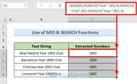
=MID(B5,SEARCH("Year ",B5)+4,SEARCH(" Club",B5)-SEARCH("Year ",B5)-4)- Hit Enter.
- In cell C5 we can see the value of the number part from the string of cell B5 after the text Year.
- Drag the Fill Handle tool from cell C5 to C8.
- Get the result like the following image.
How Does the Formula Work?
- SEARCH(“Year “,B5): The SEARCH function returns the location of string Year inside the sting of cell B5.
- SEARCH(” Club”,B5)-SEARCH(“Year “,B5)-4: This part counts the characters between the strings Club and Year.
- MID(B5,SEARCH(“Year “,B5)+4,SEARCH(” Club”,B5)-SEARCH(“Year “,B5)-4): The MID function returns the number part between the strings Year and Club.
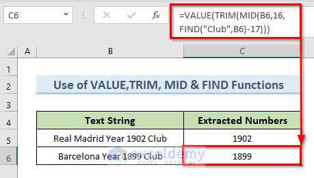
1.4 Combination of VALUE, TRIM, MID, & FIND Functions
STEPS:
- Select cell C5.
- Insert the following formula in that cell:
=VALUE(TRIM(MID(B5,18,FIND("Club",B5)-19)))- Press Enter.
- In cell C5 we get the numbers between the strings Year and Club of cell B5.
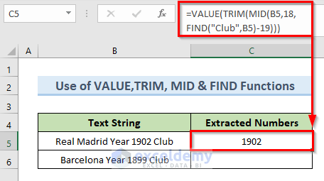
- Apply it to cell B6 also insert the following formula in cell C6:
=VALUE(TRIM(MID(B6,16,FIND("Club",B6)-17)))- Hit Enter.
- Get the result like the following image.
How Does the Formula Work?
- FIND(“Club”,B6): The FIND function finds the position of string Club in cell B6.
- MID(B6,16,FIND(“Club”,B6)-17): The MID function selects the values from the 16th character until the string Club.
- TRIM(MID(B6,16,FIND(“Club”,B6)-17))): TRIM function extracts the return portion defined by the previous part.
- VALUE(TRIM(MID(B6,16,FIND(“Club”,B6)-17))): The VALUE function in this part returns the numeric part of cell B6 in cell C6.
Method 2 – Use VBA Code to Extract Numbers after a Specific Text in Excel
STEPS:
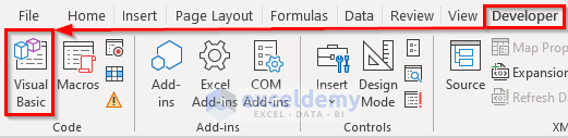
- Go to the Developer tab.
- Select the option ‘Visual Basic’.
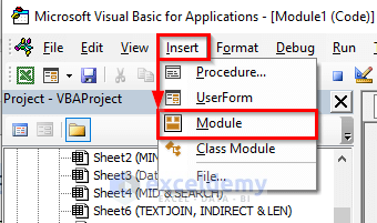
- From the VBA code window, select the Insert. From the menu, click Module.
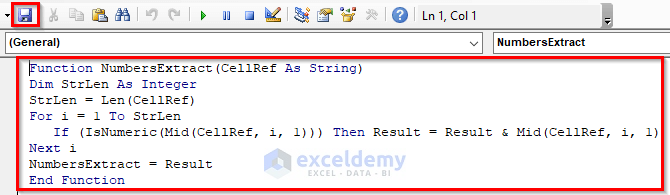
- In the blank VBA code window, type the following code:
Function NumbersExtract(CellRef As String)
Dim StrLen As Integer
StrLen = Len(CellRef)
For i = 1 To StrLen
If (IsNumeric(Mid(CellRef, i, 1))) Then Result = Result & Mid(CellRef, i, 1)
Next i
NumbersExtract = Result
End Function- Click on the save button to save the code.
- The above code creates a user-defined function named NumberExtract to extract numbers after a specific text.
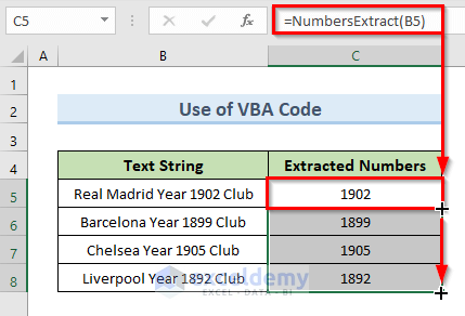
- Select cell C5. Type the user-defined function in cell C5 in the following way:
=NumbersExtract(B5)- Press Enter.
- See the numbers of cell B5 after the text Year in cell C5.
- Auto-fill the data and drag the Fill Handle tool from cell C5 to C8.
- Get results like the following image.
Extract Numbers If They Appear at the End of Text Every Time in Excel
Method 1 – Combine MIN, FIND & RIGHT Functions to Extract Numbers
STEPS:
- Insert a new column named Position.
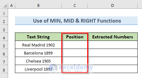
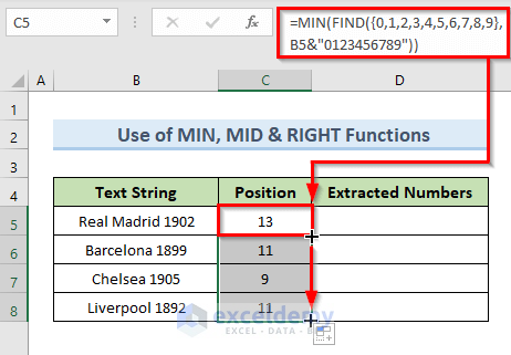
- Select cell C5. Type the following formula in that cell:
=MIN(FIND({0,1,2,3,4,5,6,7,8,9},B5&"0123456789"))- Press Enter. This action returns the starting position of the number in the string in cell C5.
- Autofill the dataset, and drag the Fill Handle tool from cell C5 to C8.
How Does the Formula Work?
- FIND({0,1,2,3,4,5,6,7,8,9},B5&”0123456789″): The FIND function finds the numeric parts in cell B5.
- MIN(FIND({0,1,2,3,4,5,6,7,8,9},B5&”0123456789″)): The MIN function returns the first position of numbers in the text string of cell B5.
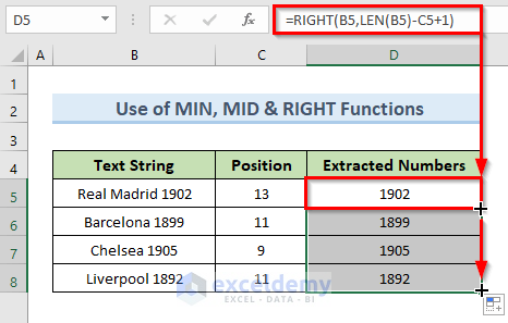
- Select cell D5. Insert the following formula in that cell:
=RIGHT(B5,LEN(B5)-C5+1)- Press Enter.
- In cell D5 we get the value of the extracted numbers from a string in cell B5.
- Drag the Fill Handle tool from cell D5 to D8 to autofill the dataset.
- Get the results like the following image.
How Does the Formula Work?
- LEN(B5)-C5+1: The LEN function returns the length of cell B5. Subtract the value of cell C5 and add 1 with the value of LEN(B5).
- RIGHT(B5,LEN(B5)-C5+1): The RIGHT function returns the strings after the position returned by the part LEN(B5)-C5+1.
Method 2 – Split Numbers with Excel SUBSTITUTE, LEFT, MIN & FIND Functions
STEPS:
- Select cell C5.
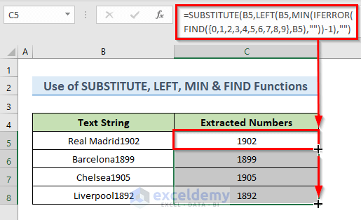
- Type the following formula in that cell:
=SUBSTITUTE(B5,LEFT(B5,MIN(IFERROR(FIND({0,1,2,3,4,5,6,7,8,9},B5),""))-1),"")- Hit Enter.
- In cell C5 the above action returns only the number part from the string of cell B5.
- Autofill, the remaining part, drag the Fill Handle tool from cell C5 to C8.
- See the result in the image below. We get all the number of parts from strings of cells (B5:B8) in cells (C5:C8).
How Does the Formula Work?
- FIND({0,1,2,3,4,5,6,7,8,9},B5): The FIND function in this part finds the numeric parts in cell B5.
- IFERROR(FIND({0,1,2,3,4,5,6,7,8,9},B5),””): If the FIND function returns any error value the IFERROR function returns a blank value.
- MIN(IFERROR(FIND({0,1,2,3,4,5,6,7,8,9},B5),””))-1): The MIN function in this part returns the least position of number from the string in cell B5. In our example is 12.
- LEFT(B5,MIN(IFERROR(FIND({0,1,2,3,4,5,6,7,8,9},B5),””))-1): Here, the LEFT function extracts 12 characters from the string in cell B5.
- SUBSTITUTE(B5,LEFT(B5,MIN(IFERROR(FIND({0,1,2,3,4,5,6,7,8,9},B5),””))-1),””): The SUBSTITUTE function substitutes the 12 characters with blank value and returns only the number parts.
Method 3 – Use Flash Fill Feature to Extract Numbers If They Appear at End of Text in Excel
STEPS:
- In cell C5 insert manually the value of the number part of the string in cell B5.
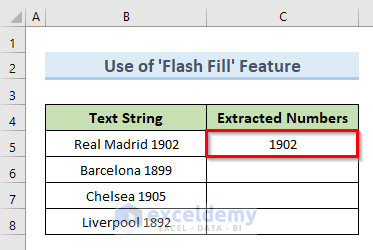
- Type the number part of the next cell.
- If Excel detects a pattern, a preview of data to be auto-filled in the cells below will appear.
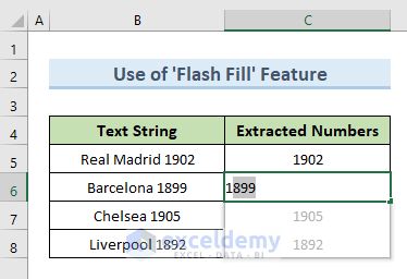
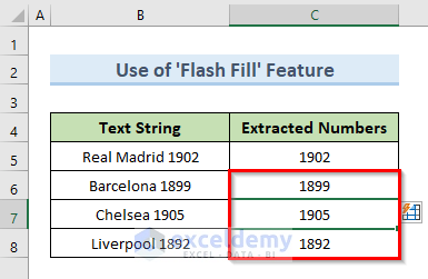
- Accept the suggestions and press Enter.
- See our desired output in the following image.
Download Practice Workbook
You can download the practice workbook from here.
<< Go Back to Separate Numbers Text | Split | Learn Excel
Get FREE Advanced Excel Exercises with Solutions!
