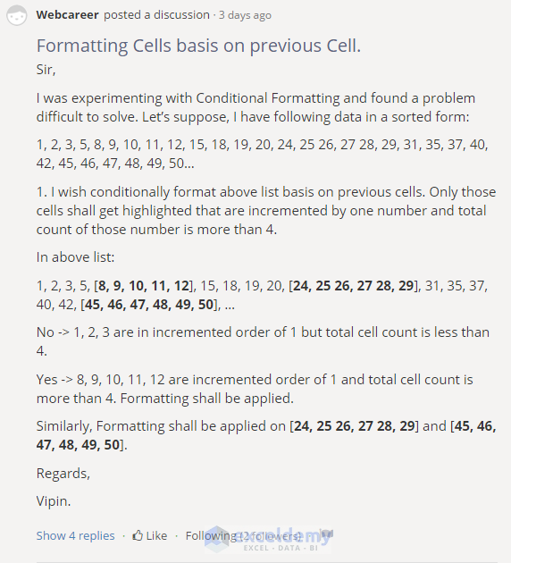
Example 1 – Applying Combined Functions to Make a FOR Loop in Excel
Here’s an overview of the problem we’ll solve with a for loop.
Steps:
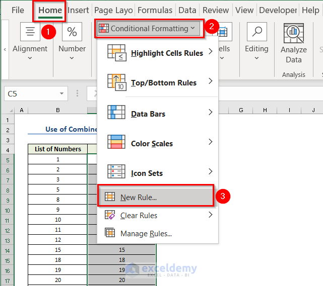
- Open a new workbook and input the above values one by one into the worksheet (start from cell C5).
- Select the whole range C5:C34.
- From the Home ribbon, click on the Conditional Formatting command.
- Select the New Rule option from the drop-down.
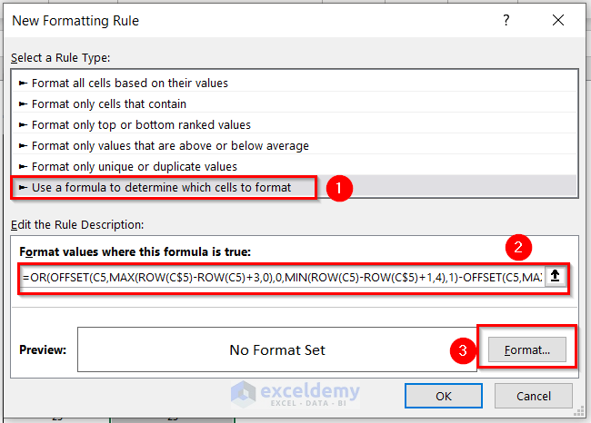
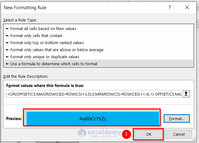
- In the Select a Rule Type window, select Use a formula to determine which cells to format option.
- In the Format values where this formula is true field, insert this formula:
=OR(OFFSET(C5,MAX(ROW(C$5)-ROW(C5)+3,0),0,MIN(ROW(C5)-ROW(C$5)+1,4),1)-OFFSET(C5,MAX(ROW($C$5)-ROW(C5),-3),0,MIN(ROW(C5)-ROW(C$5)+1,4),1)=3)- Select the appropriate format type by clicking on the Format… button in the dialog box.
- From the Fill option, choose any of the colors. We selected the Light Blue background.
- Press OK to apply the formatting.
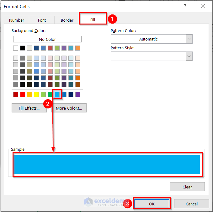
- You can see the sample in the Preview box.
- Press OK on the New Formatting Rule dialog box.
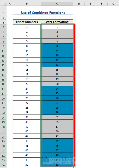
- You will get the formatted numbers.
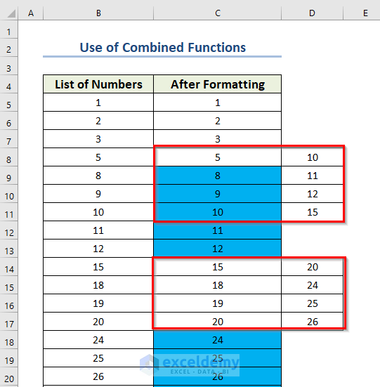
- In cells C11 and C17, the values are 10 and 20, respectively.
- We’re taking the values of cell ranges C8:C11 and C11:C14, and C14:C17 and C17:C20 side by side [image below]. Reference cells are C11 and C17 and we’re taking a total of 7 cells around the reference cell. You will get an imaginary picture like the following. From the first part, you can find a pattern from the image. C9–C12=3, C10-C13=3, there is a pattern. But for the second part, there is no such pattern.
- Before building the common formula, we’ll show what the formulas will be for the cells C11 and C17 and then will modify the formula to make it common for all. For a reference point (like C11 or C17), we need a total of 7 cells around it (including the reference point) and place them side by side in the formula creating arrays. Then we find out the difference of the arrays. If any of the differences is equal to 3, the reference cell will be TRUE-valued.
- For cell reference C11, we can write the formula like this: =OR(OFFSET(C11, 0, 0, 4, 1)-OFFSET(C11, -3, 0, 4, 1)=3). What will this formula return? The first offset function of the formula will return the array: {10; 11; 12; 15}, the second offset function will return the array {5; 8; 9; 10}. After that: {10; 11; 12; 15} – {5; 8; 9; 10} = {10-5; 11-8; 12-9; 15-10} = {5; 3; 3; 5}. When this array is logically tested with =3 Excel calculates {5=3; 3=3; 3=3; 5=3} = {False; True; True; False}. When the OR function is applied on this array: OR({False; True; False; True}, you get TRUE. Cell C11 gets TRUE.
- This formula can work from cell C8, since there are 3 cells above it. But for cells C5, C6, and C7 this formula cannot work. For cells C5 to C7, the formula will not take into consideration the upper 3 cells.
- For cell C5, the formula will be: OR(OFFSET(C5, 3, 0, 1, 1)-OFFSET(C5, 0, 0, 1, 1)=3).
- For cell C6, the formula will be: OR(OFFSET(C6, 2, 0, 2, 1)-OFFSET(C6, -1, 0, 2, 1)=3).
- For cell C7, the formula will be: OR(OFFSET(C7, 1, 0, 3, 1)-OFFSET(C7, -2, 0, 3, 1)=3).
- For cell C8, the formula will be: OR(OFFSET(C8, 0, 0, 4, 1)-OFFSET(C8,-3, 0, 4, 1)=3) (this is the general formula).
- The first OFFSET function’s rows argument has decreased from 3 to 0; the height argument has increased from 1 to 4. The second OFFSET function’s rows argument has decreased from 0 to -3 and height argument has increased from 1 to 4.
- The first OFFSET function’s rows argument will be modified like this: MAX(ROW(C$5)-ROW(C5)+3,0)
- The second OFFSET function’s rows argument will be modified like this: MAX(ROW(C$5)-ROW(C5),-3)
- The first OFFSET function’s height argument will be modified like this: MIN(ROW(C5)-ROW(C$5)+1,4)
- The second OFFSET function’s height argument will be modified like this: MIN(ROW(C5)-ROW(C$5)+1,4)
- All these four modifications are working as FOR LOOP of Excel VBA but built with Excel Formulas.
Read More: How to Create a Complex Formula in Excel
Example 2 – Use IF and OR Functions to Create a FOR Loop in Excel
We want to check if the cells contain any values or not.
Steps:
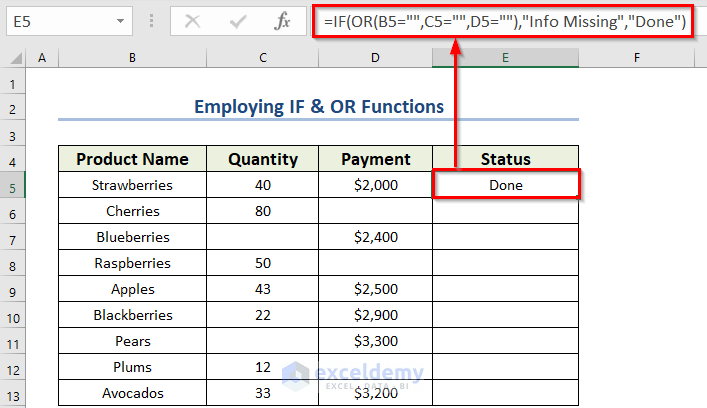
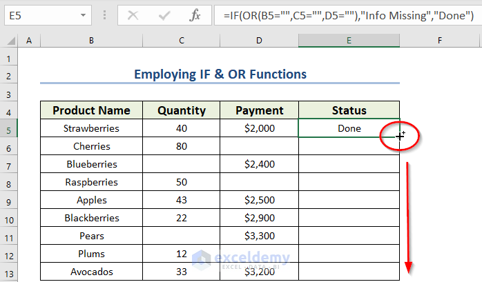
- Select cell E5 where you want to see the Status.
- Use the corresponding formula in the E5 cell.
=IF(OR(B5="",C5="",D5=""),"Info Missing","Done")- Press Enter to get the result.
Formula Breakdown
The OR function will return TRUE if any of the given logic becomes TRUE.
- B5=”” is the 1st logic, which will check whether the cell B5 contains any value.
- C5=”” is the 2nd logic, which will check whether the cell C5 contains any value.
- D5=”” is the 3rd logic. It will check whether the cell D5 contains any value.
- The IF function returns the result which will fulfill a given condition.
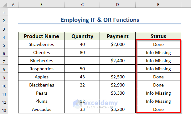
- When the OR function gives TRUE, you will get “Info Missing” as Status. Otherwise, you will get “Done” as the Status.
- Drag the Fill Handle icon to AutoFill the corresponding data in the rest of the cells E6:E13. Alternatively, double-click on the Fill Handle icon.
- You will get all the results.
Read More: How to Apply Same Formula to Multiple Cells in Excel
Method 3 – Using the SUMIFS Function to Create a FOR Loop in Excel
We want to make the total bill for a certain person.
Steps:
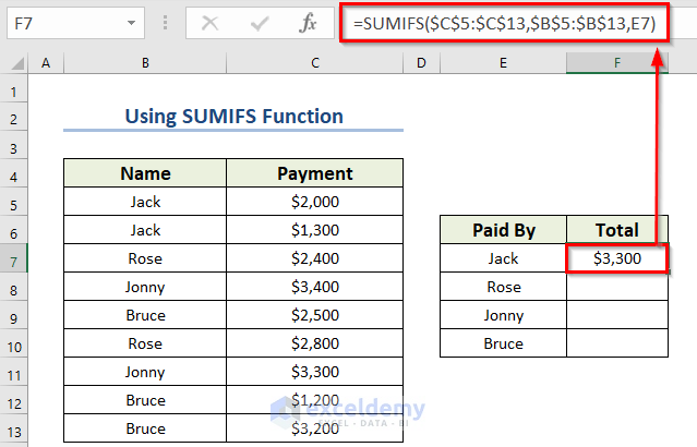
- Select cell F7 where you want to see the Status.
- Use the corresponding formula in the F7 cell.
=SUMIFS($C$5:$C$13,$B$5:$B$13,E7)- Press Enter to get the result.
Formula Breakdown
- $C$5:$C$13 is the data range from which the SUMIFS function will do the summation.
- $B$5:$B$13 is the data range from where the SUMIFS function will check the given criteria
- E7 is the criteria.
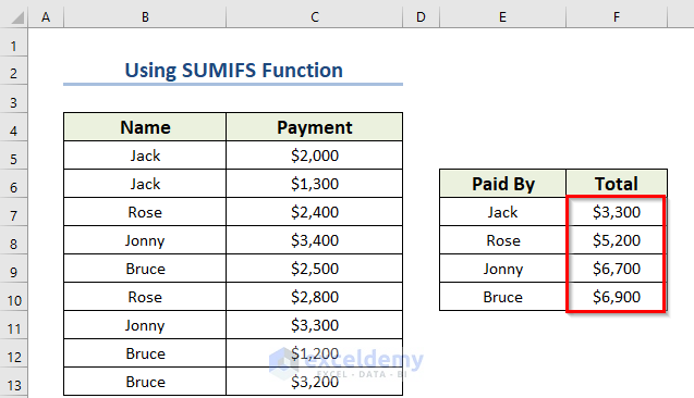
- The SUMIFS function will add the payments for the E7 cell value.
- Drag the Fill Handle icon to AutoFill the corresponding data in the rest of the cells F8:F10.
Download the Practice Workbook
Related articles
- How to Use Multiple Excel Formulas in One Cell
- How to Apply Formula to Entire Column Without Dragging in Excel
- How to Apply a Formula to Multiple Sheets in Excel
- How to Exclude Zero Values with Formula in Excel
- How to Apply Formula to Entire Column Using Excel VBA
<< Go Back to How to Create Excel Formulas | Excel Formulas | Learn Excel
Get FREE Advanced Excel Exercises with Solutions!

Hi Kawser,
nice post. However, I couldn’t solve this loop using offset.. Any ideas?
what i’m trying to do is add the letter “A” in front of the string “BCD” until length of the string becomes 10. (for which A would need to be added 7 times in front of “BCD” to make it “AAAAAAABCD”
If cell A1 holds your string “BCD” and you want to show “AAAAAAABCD” in cell B1, input this formula in cell B1: =REPT(“A”, 10-LEN(A1))&A1.
To solve this problem, you don’t have to use any looping. Or, do you have some other requirement for this problem? Let me know.
Best regards.
hi,
Thank you for details information.
I have 2 columns of numbers , say each column 10 numbers , total 20 numbers.
I want delete the similar numbers in both columns and keep just the numbers are different. Numbers need be sorted from small to large too.
this is urgent case.
Any comment I appreciate.
Hi, BIJAN!
Thank you for your query.
You can achieve your desired result following the workflow below:
I hope, it helps.
Regards,
Tanjim Reza
can i know how can i make the rows change as per the set values. Ex:
If i entered 5, rows in excel=5 & if 6, rows in excel=6 & so on…
Hi, BANDEET POUDEL!
Thank you for your query.
I am a little bit confused about your query. Are you asking if you can jump to a row upon writing the row number at an instant?
If you are asking this, then the solution is:
You can write the preferred cell’s reference number in the name box and press the Enter button to jump there in an instant.
Please let us know the feedback if your problem is solved or if you meant some other things in your query.
Regards,
Tanjim Reza
I want to ask that if I want to use for loop in Excel to print timestamp as a data is entered in respective column but what happening is as the dates are getting changed so I want it to be different… If I entered data in 1st column the date and time should be entered automatically without using vbd how can do so?
Great formula but I can’t understand how to incorporate it into a SUMIFS formula that I need to perform a loop.
Hi, JEFF!
Thank you for your query.
I am afraid you can not incorporate this article’s formula into the SUMIFS formula to perform a loop because we have used the MAX function in this article. But, it is a limitation of Excel to use the SUMIFS function with the MAX function.
To know about some other Excel limitations, you can follow the link below:
22 Limitations of Excel That Might Frustrate You
Regards,
Tanjim Reza
I think there is a slight error in this formula, for cell A2 u r using =OR(OFFSET(A2, 3, 0, 1, 1)-OFFSET(A2, 0, 0, 1, 1)=3). It means if A5 – A2 = 3 then highlight. In the given case the first four values are 1,2,3,5 hence it worked. If the values are like 1,3,2,4 then it will not work as it highlights the cells even when they do not meet the criteria
Hi, BHANU!
Thank you for your query.
As the problem discussed here is sorted from smallest to largest, you would also need to sort your numbers before applying this article’s approach.
Regards,
Tanjim Reza
I think there is an error in the formula, for cell A2 you are using =OR(OFFSET(A2, 3, 0, 1, 1)-OFFSET(A2, 0, 0, 1, 1)=3). It means if Cell A5-A2=3 then highlight, it works for the above given data as the first four values starting from A2 are 1,2,3,5. But if the values are 1,5,2,4 (for example) it highlights them even if they do not meet the criteria.
Hi, BHANU!
Thank you for your query.
As the problem discussed here is sorted from smallest to largest, you would also need to sort your numbers before applying this article’s approach.
Regards,
Tanjim Reza
The criteria of this problem supposed that the data are sorted. Your examples aren’t in sorted order.
Hi, JAMAL!
You have pointed out the correct thing in response to BHANU’s problem.
Thank you for your valuable feedback!
Regards,
Tanjim Reza
How to subtract 2 arrays using offset?
Because when I use MAX(OFFSET(A3, 2, 0, 2, 1)-OFFSET(A3, -1, 0, 2, 1)) it isn’t working
Hi, KRISHNA!
Thank you for your query.
About your query, please check if you have put an equal sign (=) in the cell before inserting the formula. Because, on my end, your formula looks perfect. And, I checked it in my Excel sheet and it worked! If it still doesn’t work, please send us your excel file.
Regards,
Tanjim Reza
Thank you for you example. I have done something similar to cumulate a set of IDs (e.g. V1, V2, V3, V4, V7) to ranges (e.g. V1 to V4, V7).
I have a table that looks like
ID | error group 1 | error group 2 | … | error group 10
———————————————————
V1 | x1, x2 | x7 | … |
V2.1 | x2 | x1 | … |
D1 | x1 | | … | x7, x5
The number of rows in this table is known, but not fixed (normally between 10 and 100).
To Input for an existing sheet is:
error group | error | ID
1 | x1 | V1, D1
1 | x2 | V1, V2.1
2 | x1 | V2.1
2 | x7 | V1
10 | x5 | D1
10 | x7 | D1
With only 1 error type in a field of the error group I’m doing something like:
ID=IFERROR(TEXTJOIN(“, “,TRUE,FILTER(ID array ,error group 1 array=”x”,””)),””)
But I don’t know how to do for multiply error and the error code is not really fixed.
I’m not allowed to use any macro. All calculation has to be done in Excel-formulas Excel 365).
It would be nice if you give me a hint how to solve this kind of problem.
Thank you very much!
Nico
Hey NICO,
Thank you for your comment. I am replying on behalf of ExcelDemy. You can use the IF function to check through every error group. The formula will be something like this:
ID=IFERROR(IF(error group = 1,TEXTJOIN(“, “,TRUE,FILTER(ID array ,error group 1 array=”x”,””)),IF(error group = 2,TEXTJOIN(“, “,TRUE,FILTER(ID array ,error group 2 array=”x”,””)),IF(error group = 10,TEXTJOIN(“, “,TRUE,FILTER(ID array ,error group 10 array=”x”,””)),””))) ,””)I hope this will help you to solve your problem. Please let us know if you have other queries.
Regards
Mashhura Jahan
ExcelDemy.
Hi,
i want to bring characters from a cell text continue till space arrived, like if cell A1 has value Mohtasham Zaheer, then i want cell B1 carries text till occurred white space and just write Mohtasham
Dear Mohtasham,
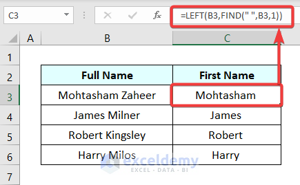
Thank you for your query. You wanted to extract a text value from a cell until a blank space appears in the text. It can be easily achieved by using a combination of LEFT function and FIND function in Excel. The formula is given below.
=LEFT(B3,FIND(” “,B3,1))
Here, we have our original text in cell B3. We applied this formula in cell C3.
The FIND function will return the position of the first space in the text of cell B3. Then, the LEFT function will extract the texts up to that position from the left side of the text. You can drag the Fill Handle to copy down the formula for other cells as well. The following image demonstrates the formula and its associated outputs.
I truly hope that this answers your question. Again thank you for reaching out to us. Please let us know in the comments area if there is anything about this approach that is unclear to you. I wish you all the best!
Regards
Zahid Hasan
ExcelDemy