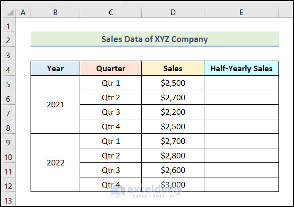
We have Sales Data of a Company as our dataset. In the dataset, we have Quarterly Sales for the Years 2021 and 2022. We will find the Half-Yearly Sales by applying formula for alternate rows.
Method 1 – Using the Fill Handle Option
Steps:
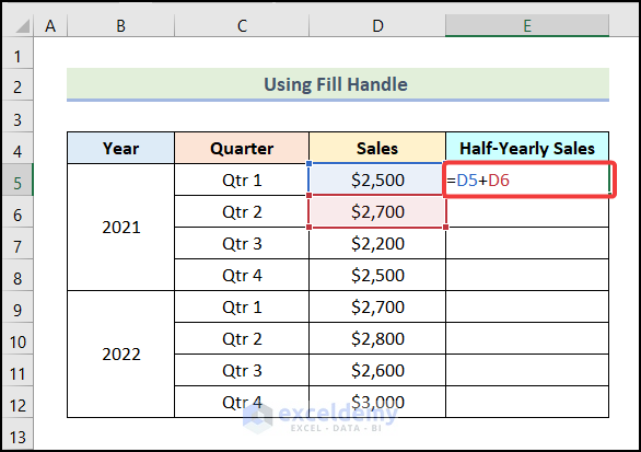
- Enter the following formula in cell E5.
=D5+D6Cell D5 represents the Sales of Qtr 1 for the Year 2021, and cell D6 refers to the Sales of Qtr 2 for the Year 2021.
- Press Enter.
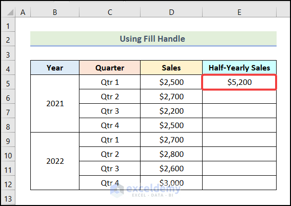
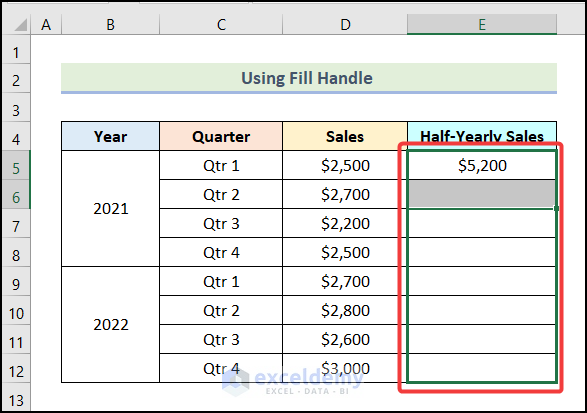
- You will have the Half-Yearly Sales for the first 2 Quarters of the Year 2021 as shown in the following picture.
- Select cell E5 along with its adjacent cell E6 as marked in the image below.
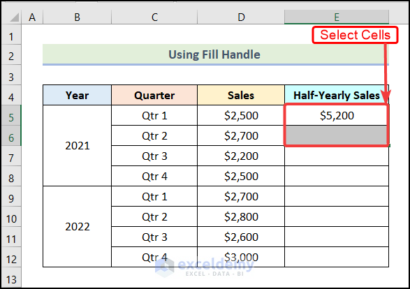
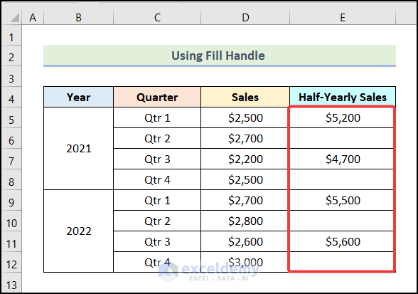
- Drag the Fill Handle down to cell E12.
- You will get the Half-Yearly Sales on the alternate rows.
Method 2 – Utilizing the Copy and Paste Command
Steps:
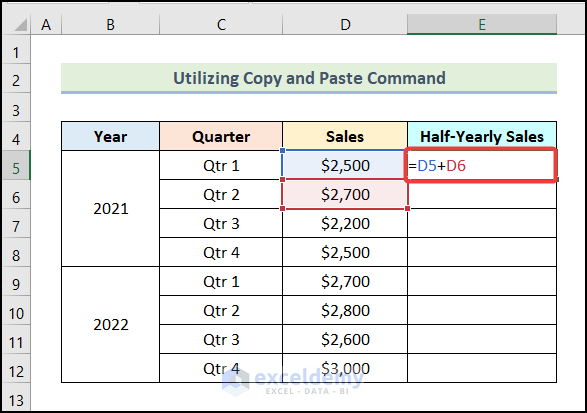
- Enter the following formula in cell E5.
=D5+D6- Hit Enter.
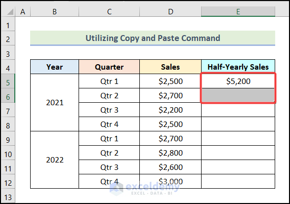
- You will get the following output on your worksheet.

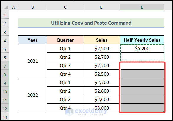
- Select cells E5 and E6 together.
- Press the keyboard shortcut Ctrl + C to copy the cells.
- Select the range of the cells where you want to apply the formula for alternate rows (the rest of the column).
- Press Ctrl + V to paste the copied cells.
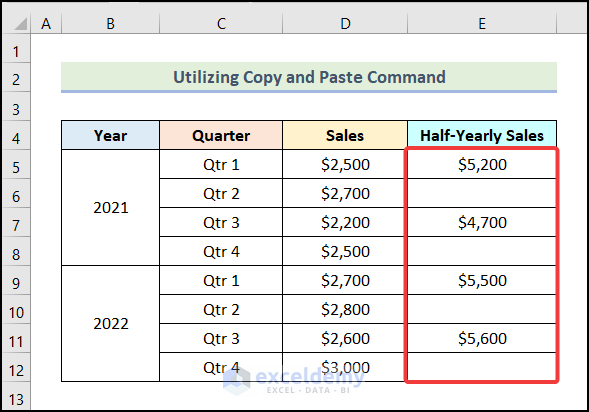
- You will get the Half-Yearly Sales in the alternate rows.
Method 3 – Using MOD and ROW Functions
Steps:
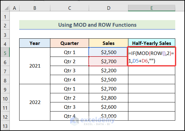
- Use the formula given below in cell E5.
=IF(MOD(ROW(),2)=1,D5+D6,"")Formula Breakdown
- ROW() → Returns the row number of a cell.
- Output → 5
- MOD(ROW(),2) → Becomes MOD(5,2)
- Returns the remainder of 5 after dividing by 2.
- Output → 1
- IF(MOD(ROW(),2)=1,D5+D6,””) → Becomes IF(1=1,D5+D6,””)
- The IF function checks whether a condition is met, and returns one value if TRUE, and another one if FALSE.
- Output → $5,200
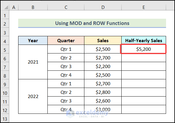
- Press Enter.
- You will get the Half-Yearly Sales for the first 2 Quarters of the Year 2021.
- Use the AutoFill feature to fill in the column.

Read More: How to Create a Custom Formula in Excel
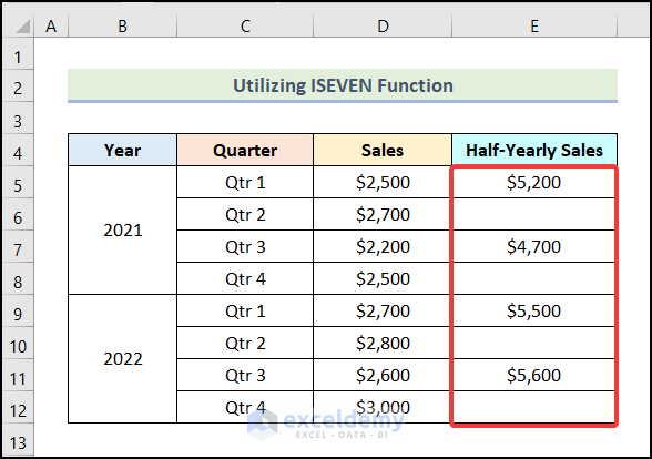
Method 4 – Utilizing the ISEVEN Function
Steps:
- Enter the following formula in cell E5.
=IF(ISEVEN(ROW())=FALSE,D5+D6,"")Formula Breakdown
- ROW() → Returns the row number of a cell.
- Output → 5
- ISEVEN(ROW()) → Becomes ISEVEN(5)
- Returns whether the number 5 is even.
- Output → FALSE
- IF(ISEVEN(ROW())=FALSE,D5+D6,””) → Becomes IF(FALSE=FALSE,D5+D6,””)
- The IF function checks whether a condition is met, and returns the second argument if TRUE, and the third one if FALSE.
- Output → $5,200
- Hit Enter.

- You will have the following output in cell E5.

- Use AutoFill for the rest of the column.
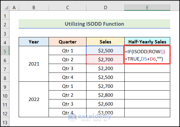
Method 5 – Using the ISODD Function
Steps:
- Use the formula given below in cell E5.
=IF(ISODD(ROW())=TRUE,D5+D6,"")Formula Breakdown
- ROW() → Returns the row number of a cell.
- Output → 5
- ISODD(ROW()) → Becomes ISODD(5)
- Returns whether the number 5 is odd.
- Output → TRUE
- IF(ISODD(ROW())=TRUE,D5+D6,””) → Becomes IF(TRUE=TRUE,D5+D6,””)
- The IF function checks whether a condition is met, and returns one value if TRUE, and another one if FALSE.
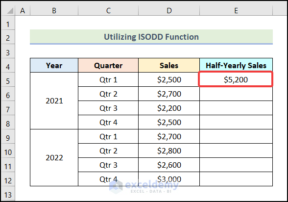
- Output → $5,200
- Press Enter.
- You will get the following output in cell E5.
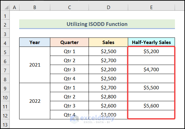
- By using the AutoFill option of Excel, you can get the rest of the outputs.
Read More: How to Create a Formula in Excel for Multiple Cells
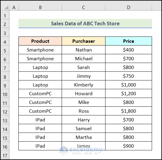
How to Color Alternate Row Color Based on Group in Excel
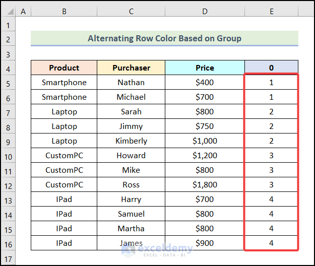
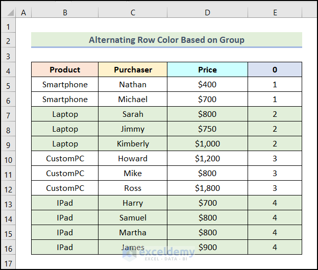
We have the Sales Data of a Store as our dataset, with Product name, Purchaser, and the Price of the Products. We need to color the alternate rows here based on the groups of Products.
Steps:
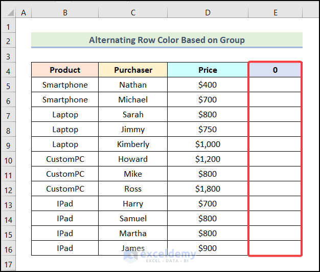
- Create a column beside the Price column and title it as 0.
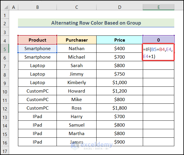
- Enter the following formula in cell E5.
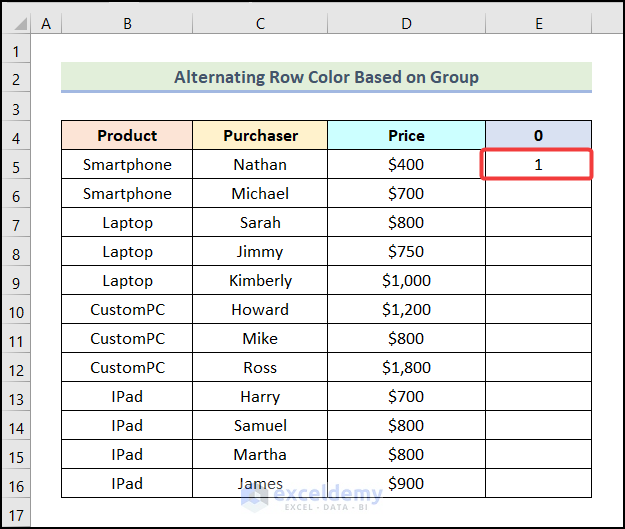
=IF(B5=B4,E4,E4+1)- Press Enter.
- Here’s the first result.
- AutoFill the column. This provides sequential group numbers.
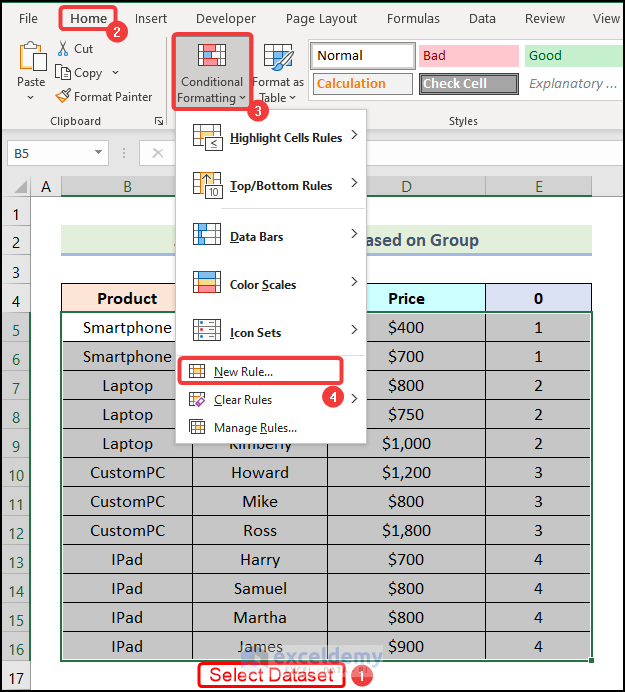
- Select the entire dataset and go to the Home tab from Ribbon.
- Choose the Conditional Formatting option from the Styles group.
- Select the New Rule option from the drop-down.
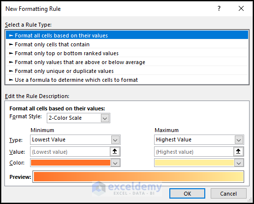
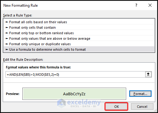
- The New Formatting Rule dialogue box will open on your worksheet.
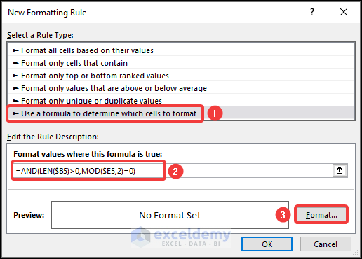
- Choose the Use a formula to determine which cells to format option.
- Enter the following formula in the field Format values where this formula is true.
=AND(LEN($B5)>0,MOD($E5,2)=0)Formula Breakdown
- LEN($B5) → Returns the length of cell B5.
- Output → 10.
- MOD($E5,2) → Returns the remainder of cell E5 after dividing by 2.
- Output → 1
- AND(LEN($B5)>0,MOD($E5,2)=0) → Becomes AND(10>0,1=0)
- The AND function checks whether all the arguments are TRUE, and returns TRUE if all arguments are TRUE. Otherwise, it returns FALSE.
- It can be written as AND(TRUE,FALSE)
- Output → FALSE.
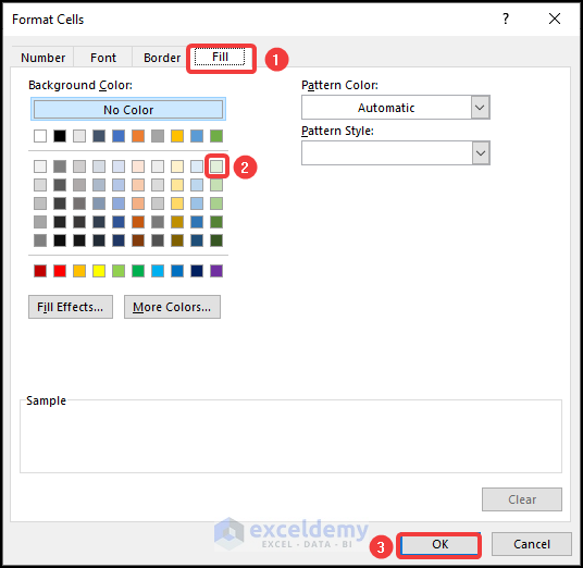
- Click on the Format option.
- Go to the Fill tab.
- Choose your preferred color and click on OK.
- You will be redirected to the New Formatting Rule dialogue box. Click on OK there.
- You will have the alternate rows colored based on group like in the following picture.
Read More: How to Create a Conditional Formula in Excel
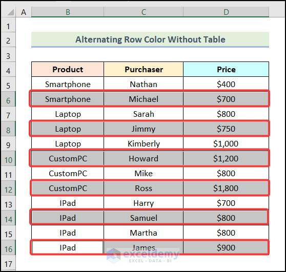
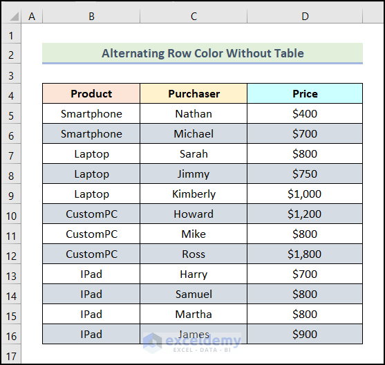
How to Color Alternate Rows Without a Table in Excel
Steps:
- Select the alternate rows while pressing the Ctrl key from your keyboard. Here, we selected rows 6, 8, 10, 12, 14, and 16.
- Go to the Home tab from Ribbon.
- Choose the Fill Color option from the Font group.
- Select your preferred color from the drop-down.
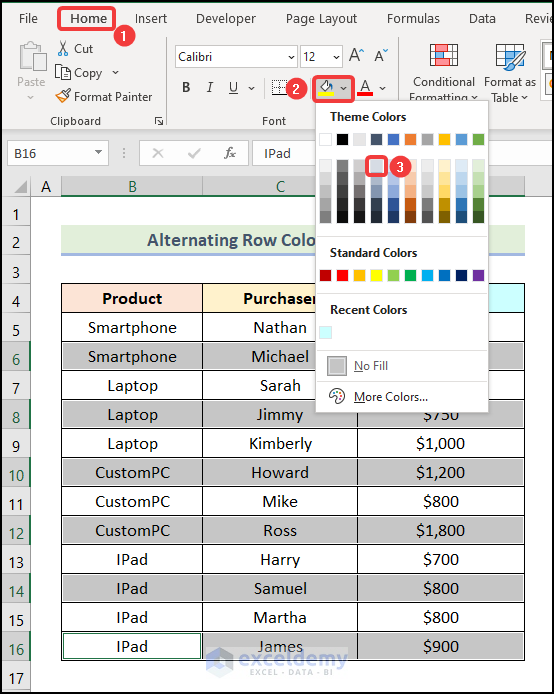
- Here’s the result.
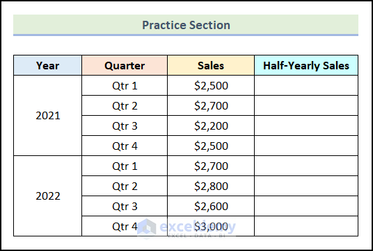
Practice Section
In the download file, we have provided a Practice Section on the right side of the worksheet.
Download the Practice Workbook
Related Articles
- How to Insert Formula for Entire Column in Excel
- How to Create a Complex Formula in Excel
- How to Create a Formula Using Defined Names in Excel
- How to Create a Formula in Excel without Using a Function
<< Go Back to How to Create Excel Formulas | Excel Formulas | Learn Excel
Get FREE Advanced Excel Exercises with Solutions!
