Let’s use a Score List of Math scores of some students. This dataset contains the ID, Student Name, and their corresponding Marks in columns B, C, and D respectively.

Method 1 – Using IF Function for a Single Condition
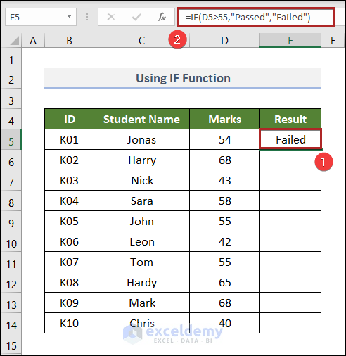
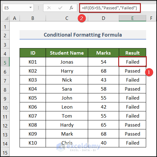
Here, we’ll check whether a student passed or failed the exam (scoring above 55 is a pass).
Steps:
- Select cell E5 and enter the formula below:
=IF(D5>55,"Passed","Failed")
Here, we applied a logical statement. If the student gets a number above 55 then the formula will return Passed in cell E5. Otherwise, it will show Failed in that cell. In this case, Jonas got 54 which is less than 55. So, she gets Failed.
- Press Enter.
- Bring the cursor to the right-bottom corner of cell E5 and it’ll look like a plus (+) sign. This is the Fill Handle tool.
- Double-click on it.
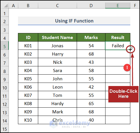
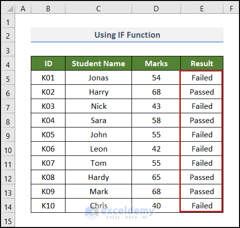
- Excel copies the formula to the lower cells and gives the output of these cells automatically.
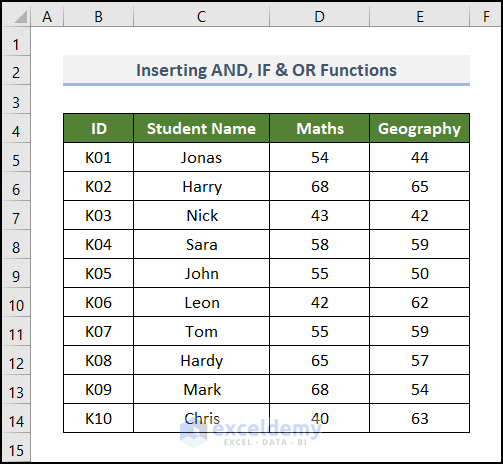
Method 2 – Inserting AND, IF, and OR Functions for Multiple Conditions
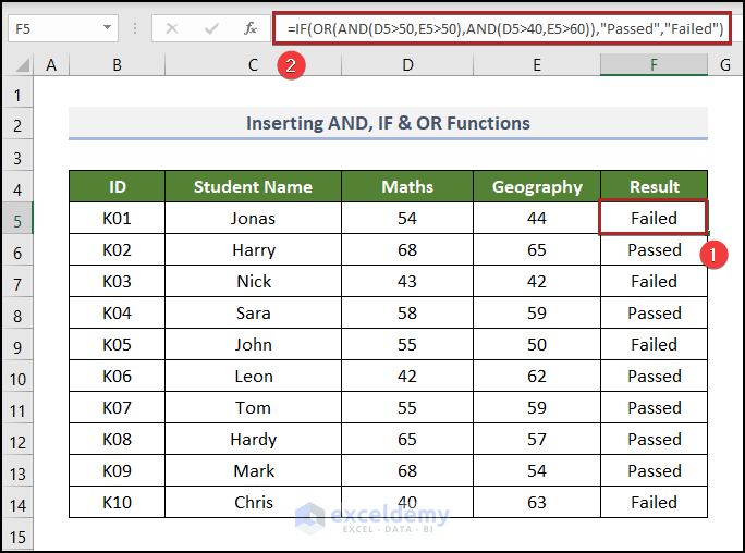
For this method, we’ll add marks for another subject: Geography. If a student gets above 50 in both subjects, he will pass the exam. Or, he has to obtain marks above 40 in Math and marks above 60 in Geography to pass the exam. Otherwise, he’ll get a “failed” result.
Steps:
- Go to cell F5 and insert the formula below:
=IF(OR(AND(D5>50,E5>50),AND(D5>40,E5>60)),"Passed","Failed")
- AND(D5>40,E5>60): This part means the marks in Maths should be above 40 and the marks in Geography should be above 60.
- AND(D5>50,E5>50): This part indicates that the number of both subjects has to be above 50.
- OR(AND(D5>50,E5>50),AND(D5>40,E5>60)): Here, the OR function checks whether any of the two arguments are TRUE.
- IF(OR(AND(D5>50,E5>50),AND(D5>40,E5>60)),”Passed”,”Failed”): If the OR function returns TRUE, then the IF function gives the output as “Passed”, otherwise it gives “Failed”.
- Press Enter.
Read More: How to Create a Formula in Excel for Multiple Cells
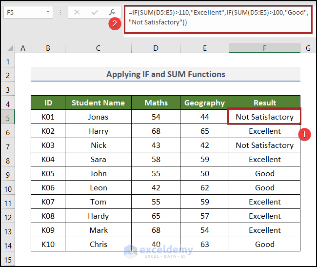
Method 3 – Applying IF and SUM Functions
Let’s score the student based on their combined scores in two subjects.
Steps:
- Select cell F5 and copy the following formula into it:
=IF(SUM(D5:E5)>110,"Excellent",IF(SUM(D5:E5)>100,"Good","Not Satisfactory"))
Here, if the sum of numbers in cells D5 and E5 is greater than 110, the formula gives the output “Excellent”. If it’s greater than 100, then the output is “Good”. Otherwise, the output is “Not Satisfactory”.
- Hit Enter.
Read More: How to Insert Formula for Entire Column in Excel
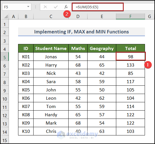
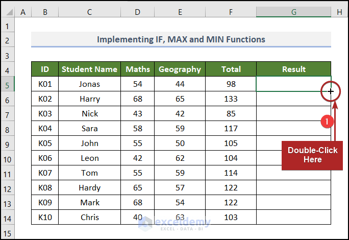
Method 4 – Implementing IF, MAX, and MIN Functions
In this example, we’ll find out who has the highest and lowest mark in the class.
Steps:
- Go to cell F5 and paste the following formula.
=SUM(D5:E5)
- Hit the Enter key.
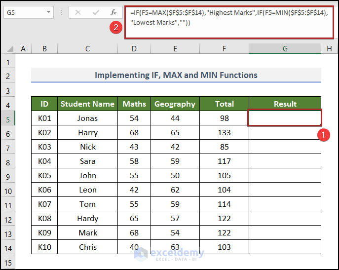
- Proceed to cell G5 and apply the formula below:
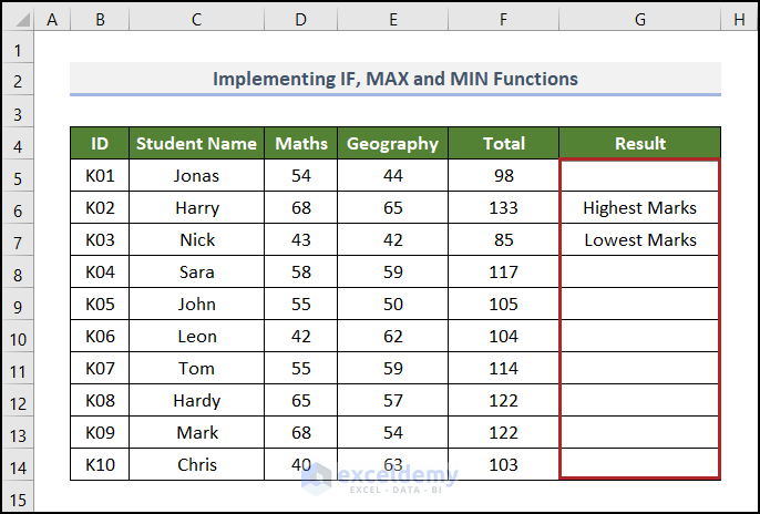
=IF(F5=MAX($F$5:$F$14),"Highest Marks",IF(F5=MIN($F$5:$F$14),"Lowest Marks",""))
In this formula, the MAX function returns the largest value in the F5:F14 range. If the total in cell F5 is equal to the largest value, then it will give the output Highest Marks in cell G5. Then, the MIN function returns the lowest value from the same range. And, if F5 is equal to the smallest value, then it will return Lowest Marks in that cell.
- Press Enter.
- Double-click on the Fill Handle tool.
- We can see that Harry gets the Highest Mark which is 133 and Nick gets the Lowest Mark which is 85.
Method 5 – Utilizing COUNTIF Function
In the following dataset, we have the respective Gender of each student. Let’s count the female students.

Steps:
- Create a new output range in the B16:D16 range.
- Go to cell D16 and put down the following formula.
=COUNTIF(D5:D14,"Female")
- Press Enter.
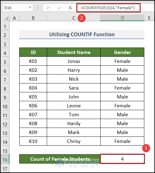
The results show that there are a total of 4 female students in the dataset. You can verify it by counting manually, as the dataset is small enough.
Creating Conditional Formatting Formula in Excel
Steps:
- Get the Results in Column E using Method 1.
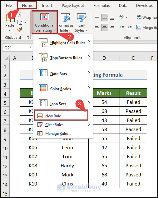
- Go to the Home tab.
- Click on the Conditional Formatting drop-down on the Styles group of commands.
- Select New Rule from the dropdown list.
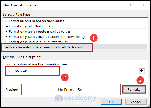
- The New Formatting Rule dialog box appears.
- Select Use a formula to determine which cells to format under the Select a Rule Type section.
- Copy the following formula in the Format values where this formula is true box:
=E5=“Passed”
- Click on the Format button.
- The Format Cells wizard pops up.
- Go to the Fill tab.
- Choose Light Green as the Background Color.
- Click OK.

- This returns to the New Formatting Rule dialog box.
- Click OK.

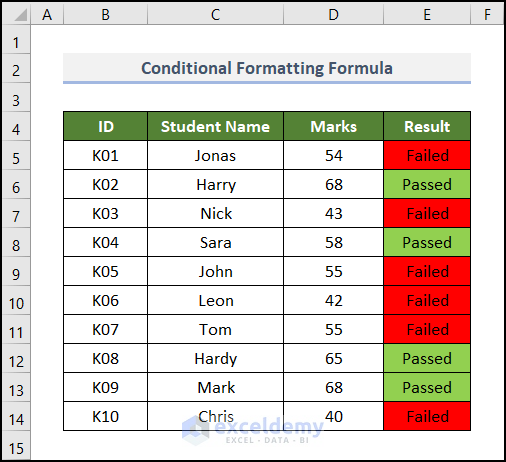
- Excel will highlight the cells containing the text Passed.
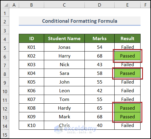
- Repeat the above steps for the cells containing Failed. Use Red as the background color in this case.
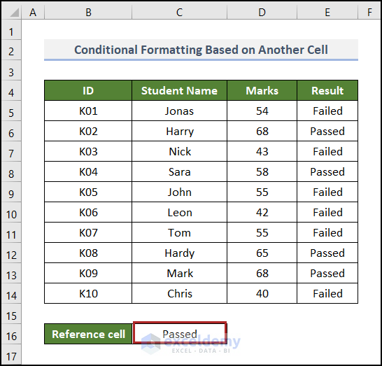
Applying Conditional Formatting Formula Based on Another Cell in Excel
Let’s apply conditional formatting in the B5:E14 range based on cell C16. The whole row will get formatted and have the “Passed” status.
Steps:
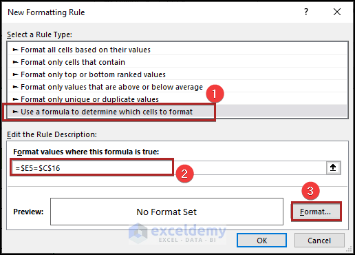
- Get to the New Formatting Rule dialog box like before.
- Select Use a formula to determine which cells to format.
- In the Format values where this formula is true box, copy the following formula:
=$E5=$C$16
- Click Format.
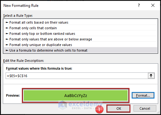
- Choose the same colors as before.
- Click OK.

- Click OK in the New Formatting Rule dialog box.
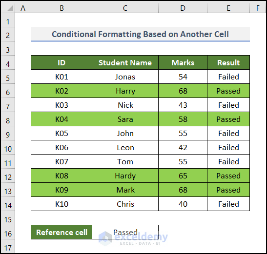
- We can see rows which contain the text Passed in the E column highlighted.
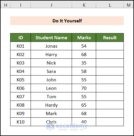
Practice Section
We have provided a Practice section like the one below on each sheet on the right side.
Download Practice Workbook
Related Articles
- How to Create a Custom Formula in Excel
- How to Apply Formula in Excel for Alternate Rows
- How to Create a Complex Formula in Excel
- How to Create a Formula Using Defined Names in Excel
- How to Create a Formula in Excel without Using a Function
<< Go Back to How to Create Excel Formulas | Excel Formulas | Learn Excel
Get FREE Advanced Excel Exercises with Solutions!
