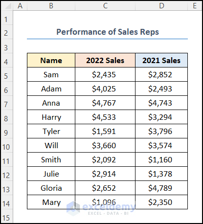
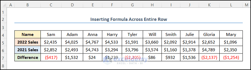
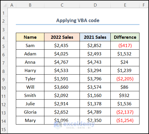
Consider the Performance of Sales Reps dataset. It showcases Names, the 2022 Sales, and the 2021 Sales of each employee.
Method 1 – Using the Fill Handle Tool
Steps:
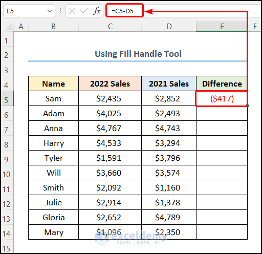
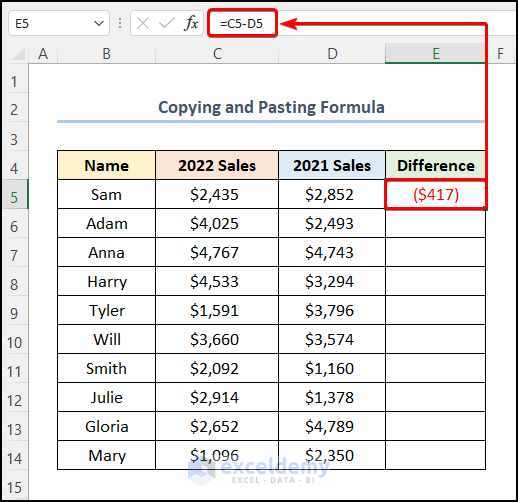
- Go to E5 >> Enter the formula below to calculate the difference in Sales.
=C5-D5
C5 and D5 are Sam’s Sales in 2022 and 2021.
- Hover the cursor at the bottom right corner of E5 >> A Plus Sign is displayed >> Drag down the cursor to copy the formula to the cells below.
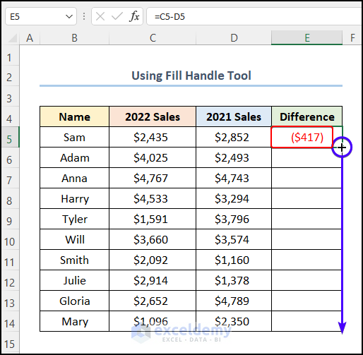
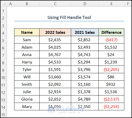
This is the output.
Read More: How to Create a Formula in Excel for Multiple Cells
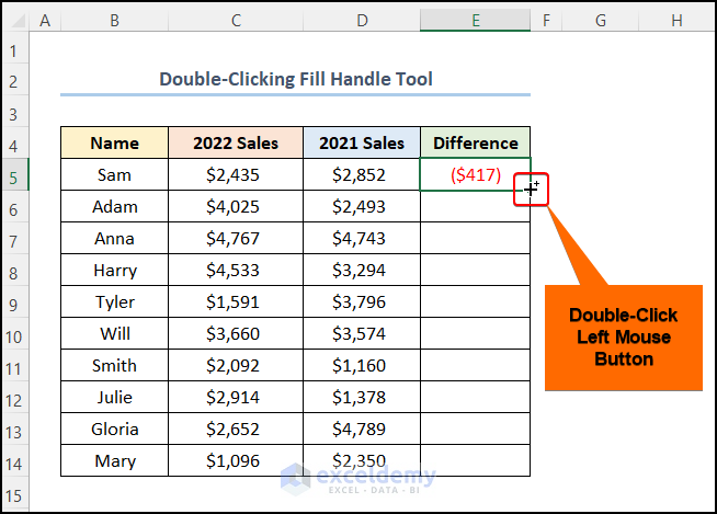
Method 2 – Double-Clicking the Fill Handle Tool
Steps:
- In E5, enter the following formula.
=C5-D5
C5 and D5 are Sam’s Sales in 2022 and 2021.

- Hover the cursor at the bottom right corner of E5 >> A Plus Sign is displayed >> Left-Click.
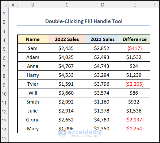
This is the output.
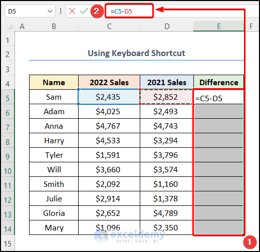
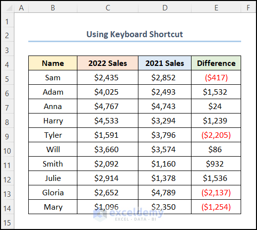
Method 3 – Applying a Keyboard Shortcut
Steps:
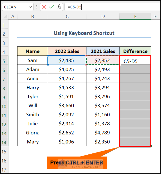
- Select E5:E14>> Enter the following formula in the Formula Bar.
=C5-D5
C5 and D5 are Sam’s Sales in 2022 and 2021.
- Press CTRL + ENTER.
This is the output.
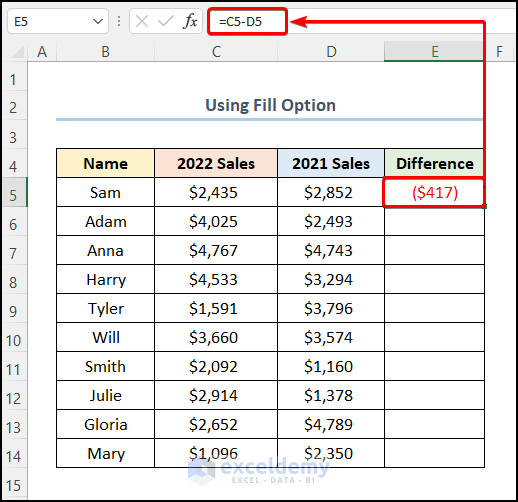
Method 4 – Utilizing the Fill Option
Steps:
- In E5, enter the following formula.
=C5-D5
- Go to Editing >> click Fill >> select Down.
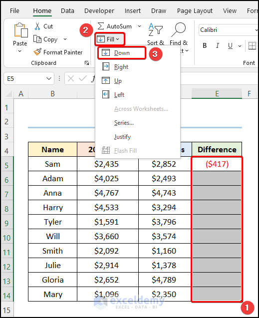
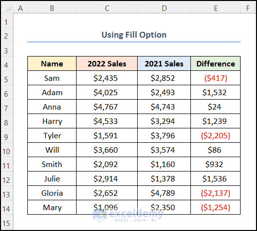
This is the output.
Method 5 – Copying and Pasting a Formula
Steps:
Calculate the difference between the 2022 and the 2021 Sales.
- In E5, enter the following formula.
=C5-D5
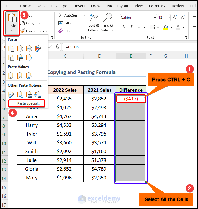
- Press CTRL + C to copy the value in E5.
- Select E5:E14 >> click Paste >> choose Paste Special.
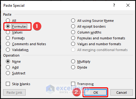
In the Paste Special dialog box:
- Select Formulas >> Click OK.
Note: You can also open the Paste Special wizard by pressing CTRL + ALT + V .
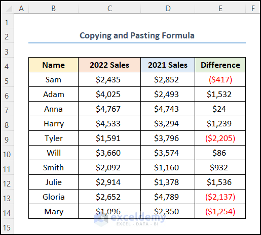
This is the output.
Method 6 – Using an Array Formula
Steps:
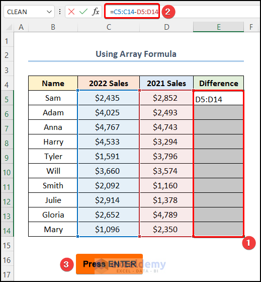
- Select E5:E14 >> Enter the formula in the Formula Bar >>Press ENTER.
=C5:C14-D5:D14
C5:C14 and D5:D14 are Sales values.
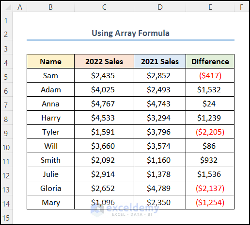
This is the output.
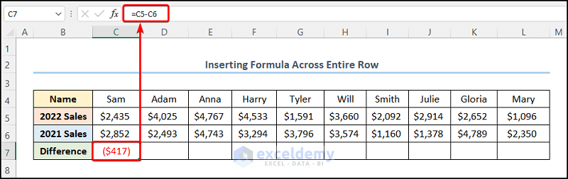
How to use a Formula for an Entire Row in Excel
Steps:
- Calculate the difference between the Sales values by subtracting C6 from C5.
=C5-C6
- Select C7:L7 and press CTRL + R.
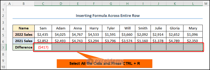
This is the output.
Read More: How to Apply Formula in Excel for Alternate Rows
Applying a Formula to an Entire Column with Excel VBA
Steps:
- Go to the Developer tab >> click Visual Basic.
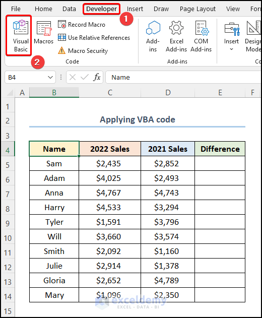
In the Visual Basic Editor window:
- Go to Insert >> select Module.
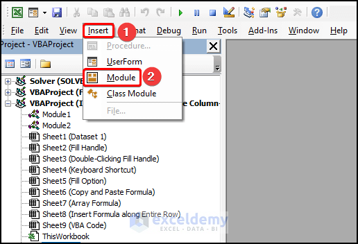
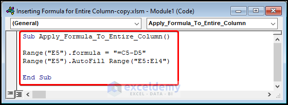
Enter the code in the window.
Sub Apply_Formula_To_Entire_Column()
Range("E5").formula = "=C5-D5"
Range("E5").AutoFill Range("E5:E14")

End Sub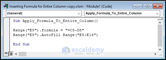
Code Breakdown:
- The sub-routine is named, here Apply_Formula_To_Entire_Column().
- The Range.formula property is used to enter a formula in the chosen range. Here, E5 using “=C5-D5”.
- The Range.AutoFill method is used to enter the formula in E5:E14.
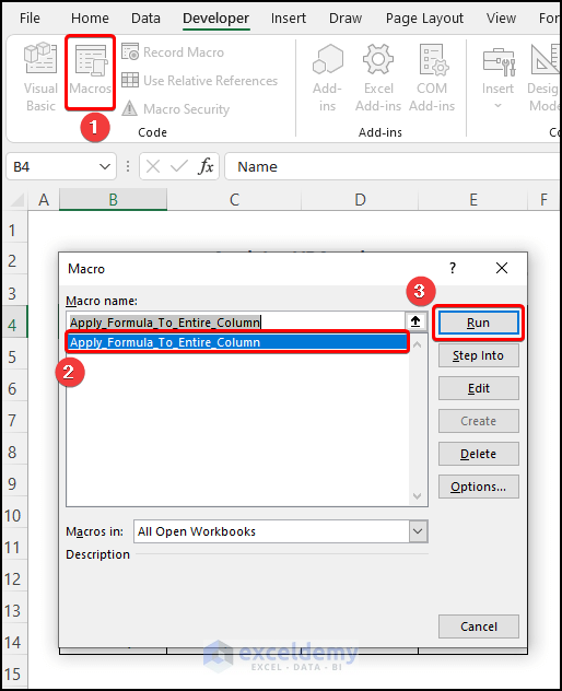
- Close the VBA window >> click Macros.
In the Macros dialog box:
- Select the copy_and_paste_data macro >> Click Run.
This is the output.
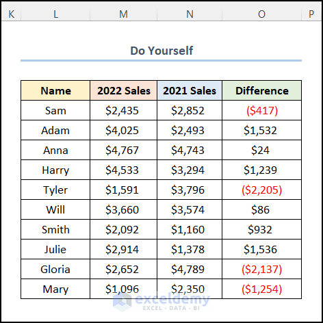
Practice Section
Practice here.
Download Practice Workbook
Download the practice workbook.
Related Articles
<< Go Back to How to Create Excel Formulas | Excel Formulas | Learn Excel
Get FREE Advanced Excel Exercises with Solutions!

I thank you for the various tips and short cuts on various topics.
You are welcome, Chandrasekhar! Glad to hear that our tips help you.
Best regards
Very useful! I knew there was a way to do this, but hadn’t taken the time to learn. Thank you!
You left out the most useful way. Convert the range to a Table first. Then add the column with the formula. Automatically the formula becomes a column formula and is applied to the entire column.
Hi Jon,
I am going to add it.
Thanks for your tips.
Best regards
Glad to know that it was helpful.
You’re welcome 🙂
Instead of Ctrl+D, just enter Ctrl+enter.
That was great man! Keep coming.
Thanks for your feedback, Mdu!
A nice option is also to put your datas in a table format and then when you input the first formula, by clicking Enter, it instantly auto fill to the bottom of the table !
Thanks for your input 🙂