Dataset Overview
Let’s consider a sales data set where sellers receive a 10% commission on each product sold. To calculate the commission, we’ve placed a formula in cell F6 (which multiplies the price in cell E4 by 0.1). We want to apply this same formula to other cells in the range F7:F18.
Note:
Remember that enabling automatic workbook calculation is essential for formulas to recalculate correctly. To enable it, go to File > Options > Formulas and choose Automatic under the Workbook Calculation section.
Applying the same formula to multiple cells streamlines calculations, reduces errors, and saves time.
Method 1 – Use the Fill Handle Tool (AutoFill Feature)
When you move your cursor to the bottom-right corner of a cell containing a formula in Excel, you’ll notice a small square known as the Fill Handle.
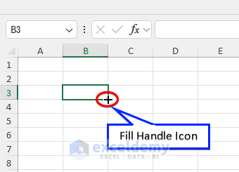
This tool allows you to quickly apply the same formula to multiple cells by dragging it in any direction. If you double-click the Fill Handle icon, it will copy the formula to contiguous cells.
If you don’t see the Fill Handle, it might be disabled. To enable it, follow these steps:
- Click on File and select Options.
- In the Excel Options window, select Advanced.
- Under Editing Options, check the Enable fill handle and cell drag-and-drop
Now, let’s consider a scenario where we want to calculate the commission for each seller. The commission rate is 10%, so the commission formula is:
Commission = Price × 10%
Additionally, we’ll calculate the gross revenue by subtracting each commission value from the respective price. Finally, we’ll determine the total values for each column.
To apply the same formula to multiple cells:
- Insert the formula in cells F6 and G6.
- Since F6 and G6 cells are contiguous and both contain the formula, select both cells.
- Hover your mouse cursor over the bottom-right corner of cell G6 (where the Fill Handle is).
- Drag the Fill Handle
- As a result, cell range F7:F18 will be filled with the same formula as cell F6, and cell range G7:G18 will be filled with the same formula as cell G6.
Similarly, you can apply the formula row-wise. For example, in cell E19, insert the formula to calculate the total. Then, drag the Fill Handle icon from cell E19 to G19 to populate the total values for each column.
Method 2 – Using the Copy-Paste Commands
You can apply the same formula to multiple cells in Excel by using copy-paste commands. Here are two ways to do it:
- Using Keyboard Shortcuts:
- Select the cells containing the formula you want to copy (e.g., F6 and G6).
- Press Ctrl+C to copy the formula.
- Select the destination cell range (e.g., F7:G18).
- Press Ctrl+V to paste the formula.
- Using Context Menu:
- Select the cells containing the formula.
- Right-click and choose Copy.
- Select the destination cell range.
- Right-click and choose Paste.
Method 3 – Use Keyboard Shortcuts
Keyboard Shortcuts for Applying the Same Value or Formula
- To apply to a range of cells: Ctrl+Enter
- To an entire column: Ctrl+D
- To an entire row: Ctrl+R
3.1 Apply Formula to a Range of Cells with Ctrl + Enter
- Select all the cells where you want to apply the formula (e.g., F6:F18).
- Go to the Formula Bar.
- Enter or paste the desired formula (e.g., =F6*0.1).
- Instead of pressing just Enter, press Ctrl+Enter.
- The formula will be applied to all cells in the selected range.
3.2 Apply Formula to Cells of a Column with Ctrl + D
Suppose you already have a formula in cell G6 (e.g., =E6-F6 for gross revenue calculation). To apply the same formula to cells in the G7:G18 range:
- Select the entire range G6:G18, including the formula cell (G6).
- Press Ctrl+D on your keyboard.
- Excel will copy the formula down the column.
3.3 Apply Formula to Cells Along a Row with Ctrl + R
If you need to apply a formula horizontally along a row:
- Select the first cell (e.g., E39) and insert the formula.
- Select the range of cells along the row where you want to apply the same formula.
- Press Ctrl+R on the keyboard.
- The formula will be applied to the selected cells in the row.
Read More: How to Apply Formula to Entire Column Without Dragging in Excel
Method 4 – Using Array Formula
You can apply the same formula to multiple cells within a range using an array formula in a single cell.
- Note 1: To apply an array formula, press Ctrl+Shift+Enter. In Excel 365, you can simply press Enter.
- Note 2: You cannot change part of the cells where you’ve applied an array formula. Any changes must be made in the first cell where the formula resides.
Follow these steps:
- Enter the following formula in the first cell (e.g., F6) to multiply all cells in the range E6:E18 by 0.1:
=E6:E18*0.1
- Press Enter (in Excel 365) or Ctrl+Shift+Enter (in previous versions of Excel).
To calculate the gross revenue, enter the following formula in cell G6:
=E6:E18 – F6:F18
In this formula, we subtract the cell range F6:F18 from E6:E18.
Note: Since F6:F18 represents an array of values, it is indicated as “F6#” to signify that it’s a dynamic array output.
Method 5 – Convert Data to Excel Table
Excel tables maintain data consistency by enforcing uniform formatting and automating formulas. When you enter a formula into a cell within an Excel table, the table automatically propagates the formula to all other cells in the same column.
To convert your dataset into a table, follow these steps:
- Click on any cell within your data.
- Press Ctrl+T. Alternatively, go to the Insert tab and select Table.
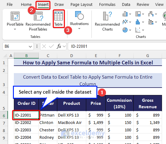
- In the Create Table dialog box that appears, verify that the selected data range is correct.
- Click OK to create your Excel table.
Now, if you insert a formula (similar to the one shown in the GIF image) into cell F6, you’ll notice that the Excel table automatically copies the formula to all other cells in that column.
Important note: Excel tables use structured references in formulas instead of conventional cell references.
To copy the formula from cell E19 to cells F18 and G18, enable the Total Row option as shown in the image.
Method 6 – Applying VBA
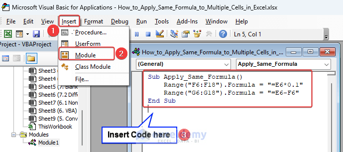
To apply the same formula to multiple cells using VBA code:
- Press Alt+F11to open the Visual Basic for Applications (VBA) editor.
- Click Insert and choose Module to create a new module.
- Copy and paste the following code into the module:
Sub Apply_Same_Formula()
    Range("F6:F18").Formula = "=E6*0.1"
    Range("G6:G18").Formula = "=E6-F6"
End Sub
- Press Alt+Q to close the VBA editor.
- To run the code, return to your worksheet, go to the Developer tab, select Macros, choose the macro named Apply_Same_Formula, and click Run.
- After running the code, you’ll see that the same formula has been inserted into the selected cell range.
Read More: How to Apply Formula to Entire Column Using Excel VBA
How to Apply Same Formula to Multiple Non-Adjacent Cells in Excel
When you need to apply the same formula to non-adjacent cells in Excel, follow these steps:
i. Cells in the Same Worksheet:
-
- Hold down the Ctrl.
- Select all the non-adjacent cells where you want to apply the formula.
- Enter the formula directly into the formula bar.
- Instead of pressing Enter, press Ctrl+Enter.
- The formula will be applied to all the selected cells.
ii. Cells in Different Worksheets (Same Positions)
- Suppose you have multiple worksheets with the same cell range (e.g., F6:F18) containing sales data for different months.
- Hold down the Ctrl.
- Select the desired worksheets by clicking on their tabs (worksheet names will turn white against a gray background).
- Enter the formula into the cells as needed.
- The same formula will now be applied across all the selected worksheets simultaneously.
How to Apply Same Formula to Multiple Cells in Excel Based on Selection
- Select the Full Dataset:
- Highlight the entire dataset where you want to apply the formula. You can do this by clicking and dragging over the cells or using keyboard shortcuts like Ctrl+A to select all cells.
- Open the “Go To” Window:
- Press F5 or use Ctrl+G to open the Go to This window allows you to navigate to specific cells or ranges within your dataset.
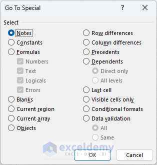
- Access the “Go to Special” Feature:
- In the Go to window, click on the Special This will open the Go to Special dialog box.
- Select Blank Cells:
- In the Go to Special dialog box, choose the Blanks option and click OK. This will select all the blank cells within your dataset.
- Enter the Formula:
- Go to the last selected blank cell (for example, cell D9).
- Enter the formula you want to apply (e.g., “=D8” if you want to refer to the previous cell).
- Press Ctrl+Enter to apply the formula to all the selected blank cells. Excel will automatically fill in the formula for each blank cell based on the pattern you specified.
By following these steps, you can quickly apply the same formula to multiple cells without manually entering it for each cell.
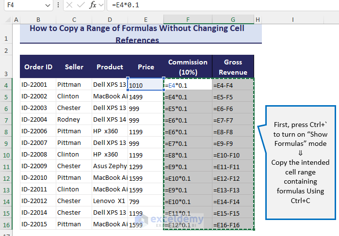
How to Copy a Range of Formulas Without Changing Cell References and Apply
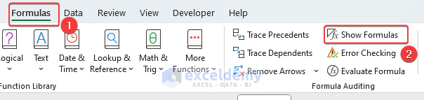
- Enable “Show Formulas” Mode:
- Press Ctrl + \ or go to the Formulas tab and click on the Show Formulas option in the Formula Auditing.
- This will display all formulas in the cells instead of their output.
- Copy the Formulas:
- Select the cell range containing the formulas you want to copy.
- Copy the selected data (either by pressing Ctrl + C or right-clicking and choosing Copy).
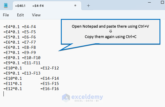
- Use Notepad as an Intermediate Step:
- Open Notepad on your device.
- Paste the copied data into Notepad.
- Copy the data again from Notepad (using Ctrl + C).
- Paste the Formulas in the Target Location:
- Return to your Excel worksheet.
- Select the target location where you want to paste the formulas.
- Keep the “Show Formulas” option turned on.
- Paste the copied data (using Ctrl + V).
- Verify that the cell references remain unchanged.
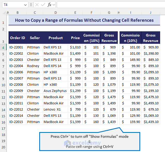
- Disable “Show Formulas” Mode:
- Press Ctrl + \ again to turn off the Show Formulas mode.
By following these steps, you’ll be able to copy formulas to a new location without altering the cell references.
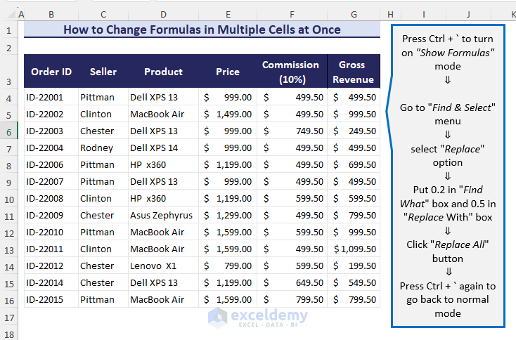
How to Change Formulas in Multiple Cells at Once
- Enable “Show Formulas” Mode:
- Press `Ctrl + “ or go to the Formulas tab in the top ribbon and click on the Show Formulas option.
- This will display all formulas in the cells instead of their output.
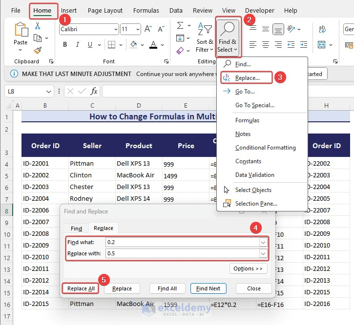
- Use Find and Replace to Update Formulas:
- Select the range of cells containing the formulas you want to change.
- Press Ctrl + H to open the Find and Replace dialog box.
- In the “Find what field, enter the formula you want to replace (e.g., C).
- Click the Options tab and select:
- Within Sheet
- By Columns
- Look In: Formulas
- Switch to the Replace tab and enter the new formula (e.g., D).
- Click Replace All.
- Any cells containing the original formula (C) will be updated to the new formula (D).
- Disable Show Formulas Mode:
- Press `Ctrl + “ again to turn off the Show Formulas option and return to normal mode.
Remember these additional tips for selecting multiple cells in Excel:
- To select a range of cells, click the first cell, hold the Shift key, and click the last cell in the range.
- To select an entire column containing the active cell, press Ctrl + Spacebar.
- To select an entire row containing the active cell, press Shift + Spacebar.
- For other selection shortcuts, such as selecting adjacent cells or the entire worksheet, use the provided keyboard combinations.
Download Practice Workbook
Related Articles
<< Go Back to How to Create Excel Formulas | Excel Formulas | Learn Excel
Get FREE Advanced Excel Exercises with Solutions!

Dear Sir, 29th Feb,2020.
Fantastic and clearly shown all examples.Appreciate your efforts to clear the ideas in details.
Rarely found such examples.
Thanking you and hope to receive more and more ideas in future too.
Kanhaiyalal Newaskar.
Good article but I have another issue perhaps you may advise I have a massive table with multiple values in each cell in the table however I would like to multiply certain cells with another cell let’s call it the value cell but rather than create another table where I can multiply these to values to get an answer I want to apply this into the table then I want to be able to tweak the value cell which should change the values I applied this formula to just imagine if I created a second table I would like to forget the second table
Thanks, RON for your amazing question. Let me help you out in solving your problem. Please follow the below steps with us.
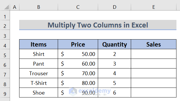
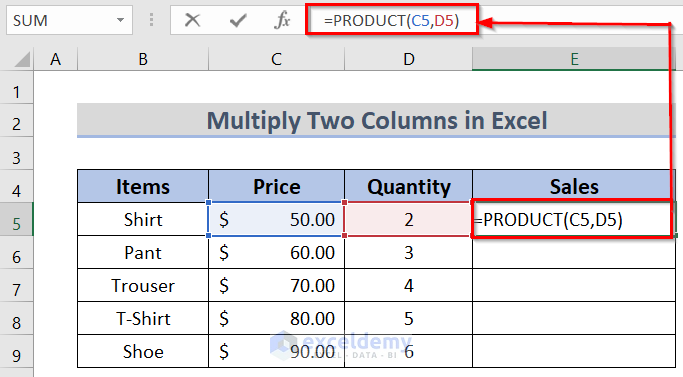
First, we arranged a dataset and add an extra column(in this case Sales) in the same table as the below image.
Then, insert the following formula in cell E5.
=PRODUCT(C5,D5)
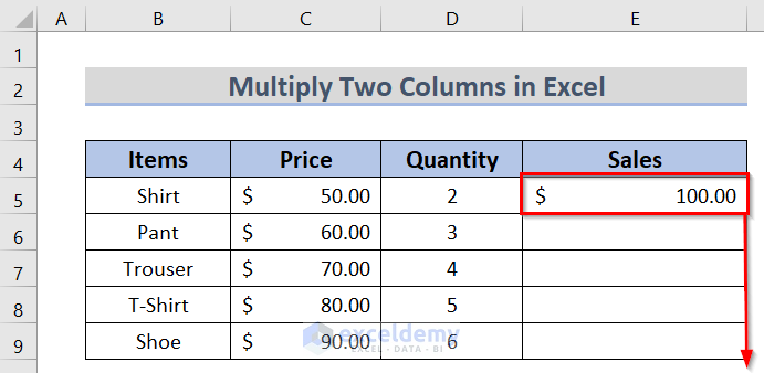
After that, if you press the Enter button, then you will get the result for that cell, and afterward, use the Fill Handle option to apply the formula to all cells.
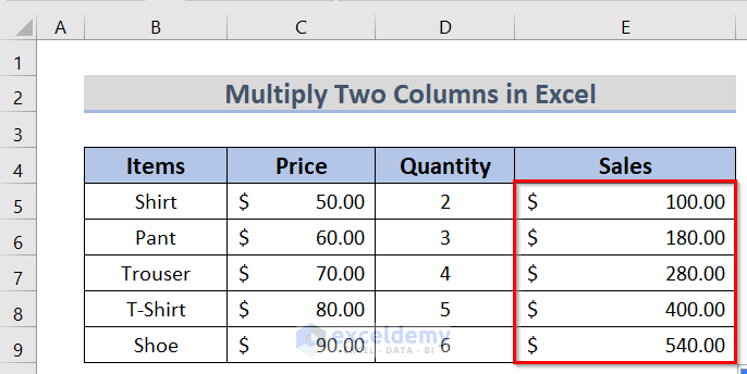
Finally, you will get the desired result.
So, I have tried to solve the problem to multiply the cells in the same table. If you face any other confusion, then we request you to provide the Excel file and give us the opportunity to help you out. All the best.