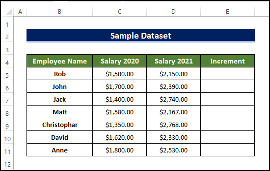
We have a dataset that contains some employees’ salaries for two years and their salary increments.
Method 1 – Use the AutoFill Tool
Steps:
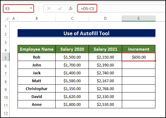
- Select cell E5 and insert the following formula:
=D5-C5
- Hit the Enter button.
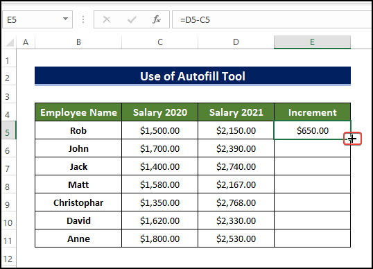
- Double-click the Plus (+) symbol (Fill Handle) at the bottom-right corner of the cell or click and drag on the Fill Handle through the cells you need.
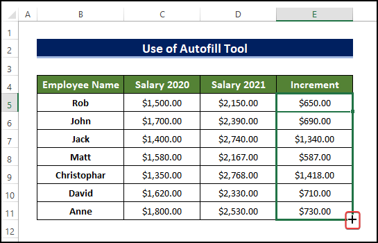
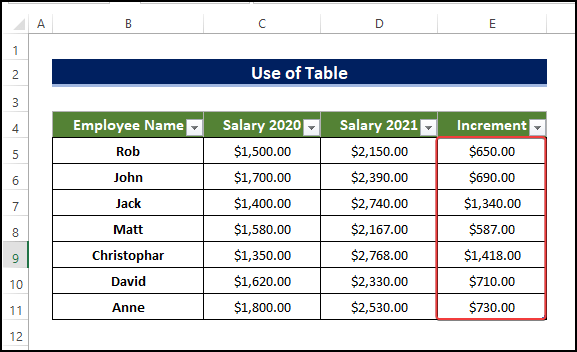
- After dragging the Fill Handle to cell E11, we can see that the range of cell E5:E11 is now filled with the increment value of salary from 2020 to 2021.
Method 2 – Input a Formula in Multiple Cells with Keyboard Shortcut
Steps:
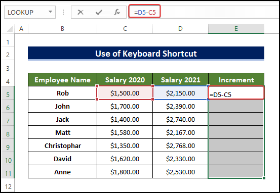
- In the cell E5, insert the following formula:
=D5-C5
- Select all the cells of the “Increment” column.
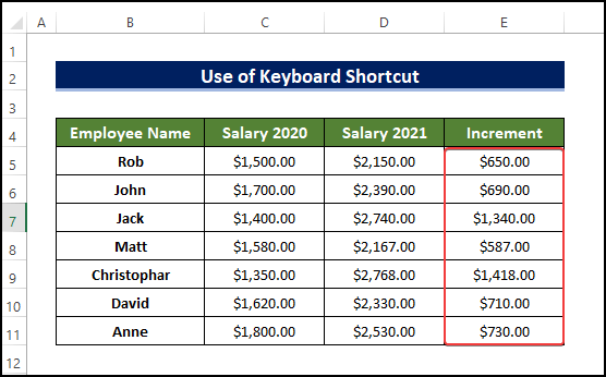
- Press Enter.
- Press Ctrl + Enter.
Read More: How to Apply Same Formula to Multiple Cells in Excel
Method 3 – Insert an Excel Table
Steps:
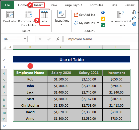
- Select your intended dataset including the headers.
- Go to Insert tab and select Table.
- You’ll get a dialog window with the preselected range.
- Check the “My table has headers” option.
- Press OK.
- Press = at cell E5.
- Select cell D5, type – and select cell C5. It will look like the image below.
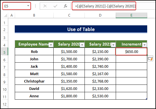
- Press the Enter button.
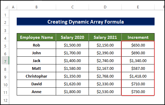
Method 4 – Create a Dynamic Array Formula
Steps:
- Select cell E5 and enter the following formula:
=D5:D11-C5:C11

Note:
Here we can manually select the arrays by typing them.
- Press the Enter button.
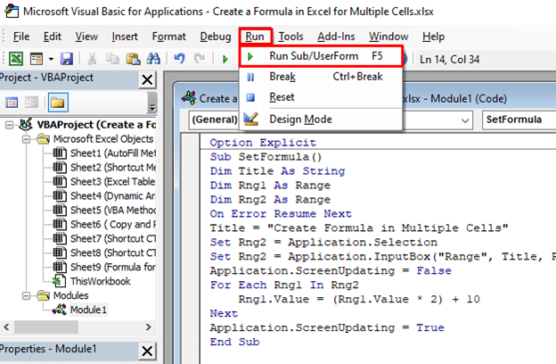
Method 5 – Embed VBA Macro
Steps:
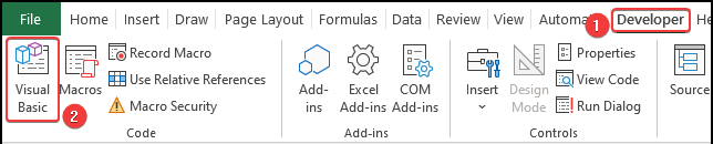
- Go to the Developer tab and click on Visual Basic. If you don’t have it, you have to enable the Developer tab, or you can press Alt + F11 to open the Visual Basic Editor.
- You’ll get a new editor box.
- Click on Insert and select Module.
- In the Module editor window, insert the following code.
Option Explicit
Sub SetFormula()
Dim Title As String
Dim Rng1 As Range
Dim Rng2 As Range
On Error Resume Next
Title = "Create Formula in Multiple Cells"
Set Rng2 = Application.Selection
Set Rng2 = Application.InputBox("Range", Title, Rng2.Address, Type:=8)
Application.ScreenUpdating = False
For Each Rng1 In Rng2
Rng1.Value = (Rng1.Value * 2) + 10
Next
Application.ScreenUpdating = True
End Sub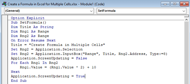
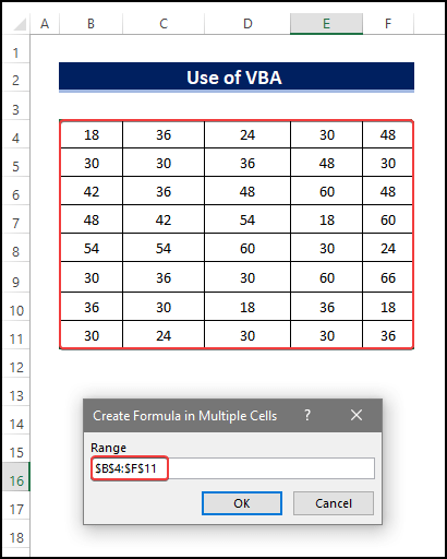
- Press the Run tab and select Run/UserForm or press F5. A dialog box will appear.
- Select the range of cells B4:F11 from the table by clicking and dragging.
- Hit OK.
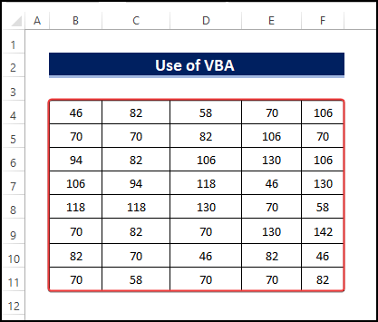
- The same formula has been applied to all the cells in the table.
Read More: How to Apply Formula to Entire Column Using Excel VBA
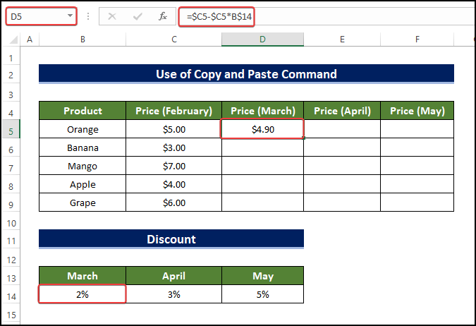
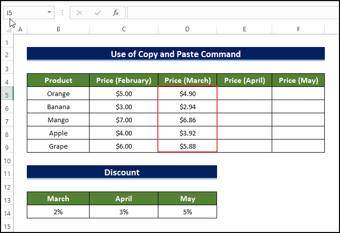
Method 6 – Use Copy and Paste
Steps:
- Use the following formula in cell D5.
=$C5-$C5*B$14
- Hit Enter.
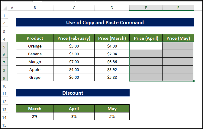
- Copy cell D5 with Ctrl + C.
- Select the range of cell D5:D9 and press Ctrl + V.
- The same formula is now copied to all the cells.
- Repeat the same process for the rest of the cells.
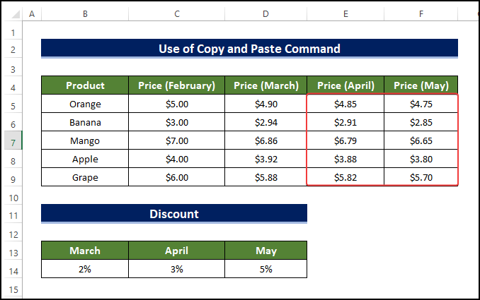
- Select cell E5:F9 and press Ctrl + V.
- Pressing the Ctrl + V will copy or replicate all the formulas in the range of cell E5:F9.
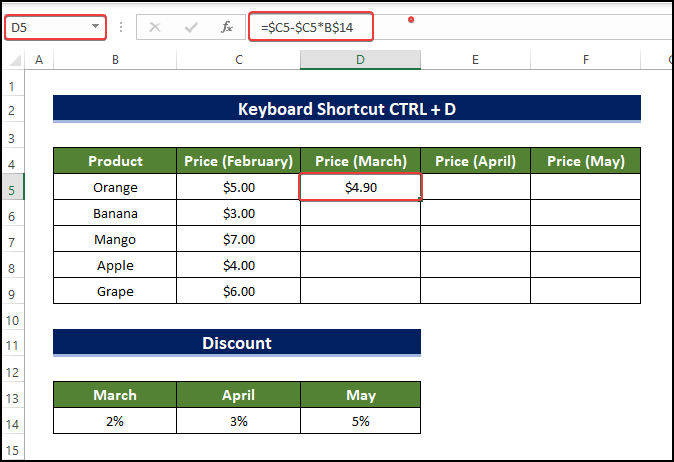
Method 7 – Utilize the Keyboard Shortcut Ctrl + D to Paste Along Columns
Steps:
- Enter the following formula in cell D5.
=$C5-$C5*B$14
- Press Enter.
- Select the range of cells containing D5:D9.
- Press Ctrl + D.
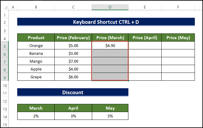
- The range of cell D5:D9 will have the formulas in the Price (March) column.
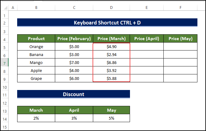
- Repeat the same process for the later months.
Note:
This method is only applicable to columns.
Method 8 – Apply the Keyboard Shortcut Ctrl + R
Steps:
- Enter the following formula in cell D5.
=$C5-$C5*B$14
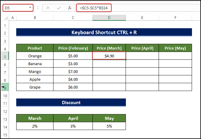
- Select the range of cells containing D5 to D9.
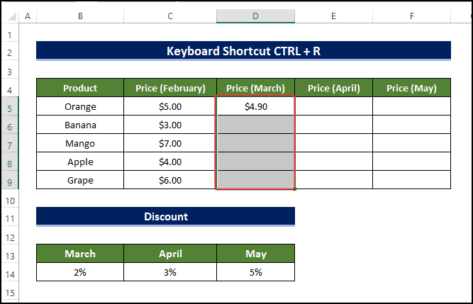
- Press Ctrl + R. The formula will be copied to the column.
- Select E5:E9 and press Ctrl + R.
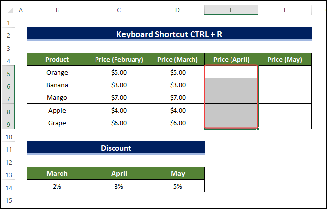
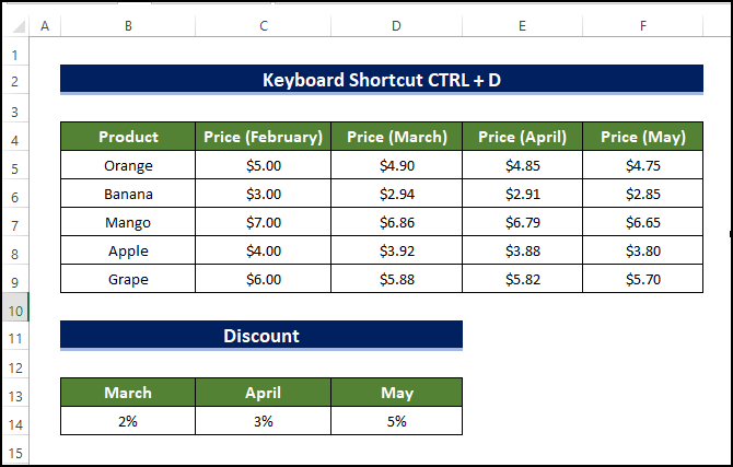
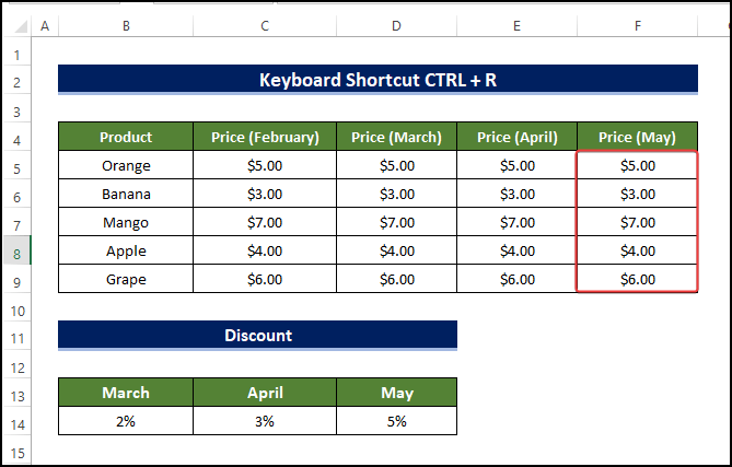
- The formulas are now filled and repeat the same process for the Price (May).
- You have the price value for each of the months in the range of cell C5:F9.
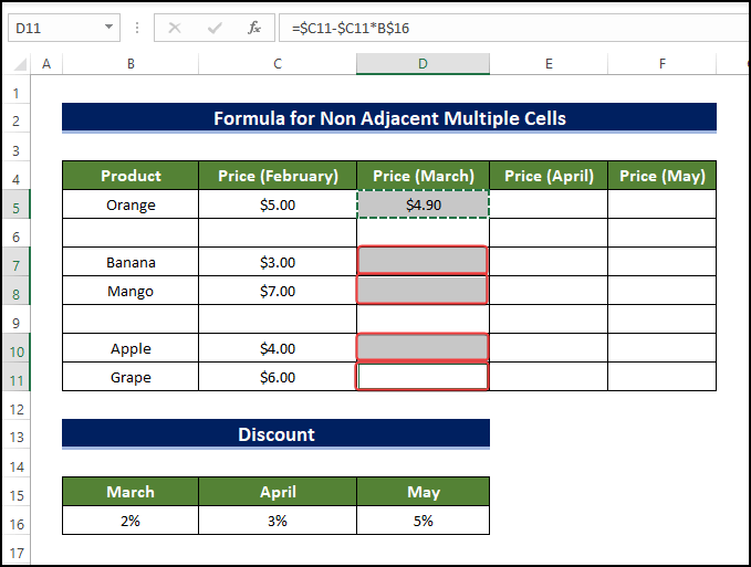
Method 9 – Input a Formula to Non-Adjacent Multiple Cells
Steps:
- Apply the following formula in cell D5.
=$C5-$C5*B$16
- Hit Enter.
- Copy cell D5.
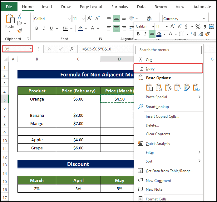
- Press and hold the Ctrl key and select the cells where you want to copy the formula as shown below.
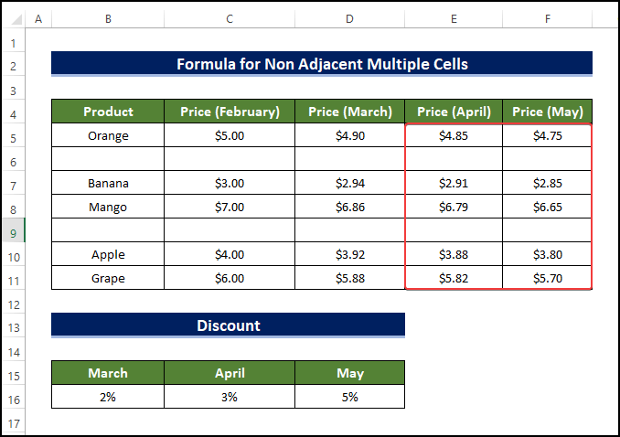
- Press Ctrl + V.
- Rrepeat the same process for the rest of the months (April and May).
Read More: How to Apply Formula in Excel for Alternate Rows
Download the Practice Workbook
Related Articles
- How to Create a Complex Formula in Excel
- How to Create a Conditional Formula in Excel
- How to Create a Formula Using Defined Names in Excel
- How to Create a Formula in Excel without Using a Function
<< Go Back to How to Create Excel Formulas | Excel Formulas | Learn Excel
Get FREE Advanced Excel Exercises with Solutions!
