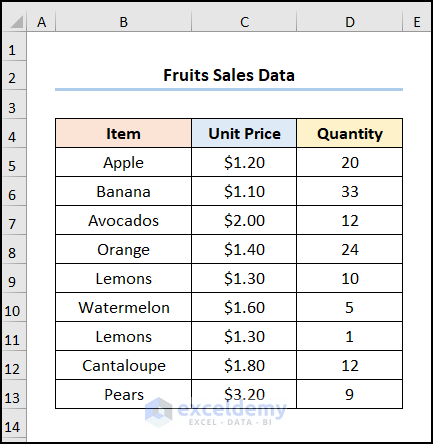
The sample dataset (B4:D13) showcases Item, Quantity, and Unit Price of Fruit Sales.
Example 1: Multiplying Named Ranges
Steps:
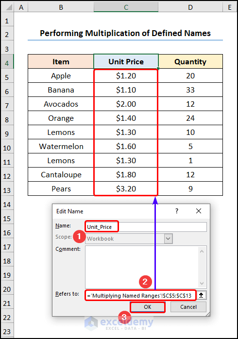
The Edit Name window will be displayed.
- In Name, enter “Unit_Price” >> in Refers to, select C5:C13 >> click OK to create a Defined Name.
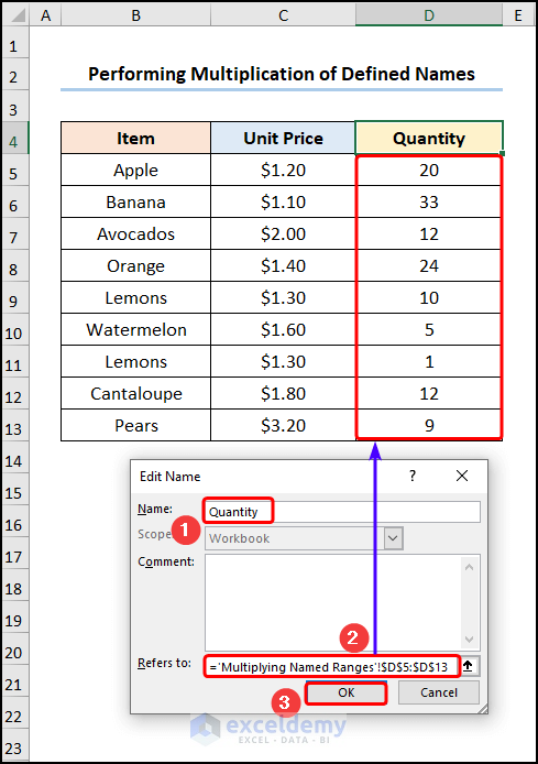
- Create a Defined Name for “Quantity” by selecting D5:D13.
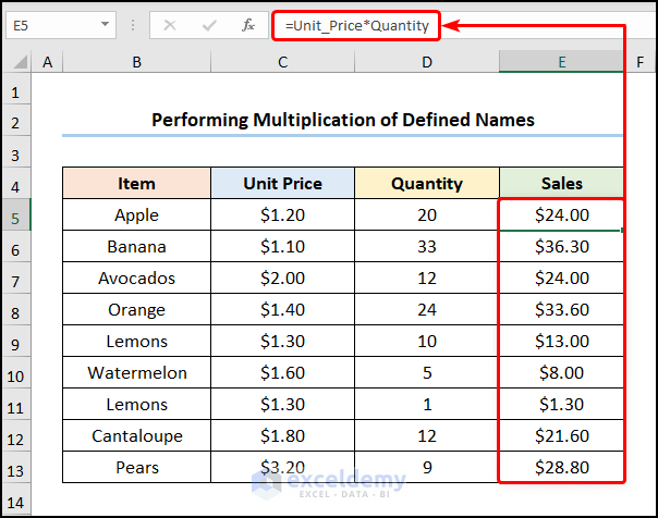
- Multiply the “Unit Price” by “Quantity” to calculate the Sales in USD.
=Unit_Price*Quantity
The “Unit_Price” and the “Quantity” refer to the Defined Names: C5:C13 and D5:D13.
Note: In Microsoft 365, you can run the Array Formula by pressing ENTER. In older versions, you must press CTRL + SHIFT + ENTER.
Read More: How to Create a Formula in Excel without Using a Function
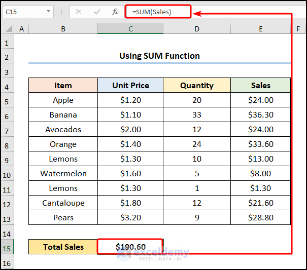
Example 2 -Using the SUM Function
Steps:
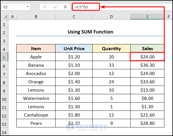
- Go to E5 >> enter the formula below.
=C5*D5
C5 and D5 cells represent “Unit Price” and “Quantity”.
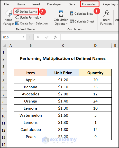
- Go to Formulas >> choose Define Name.
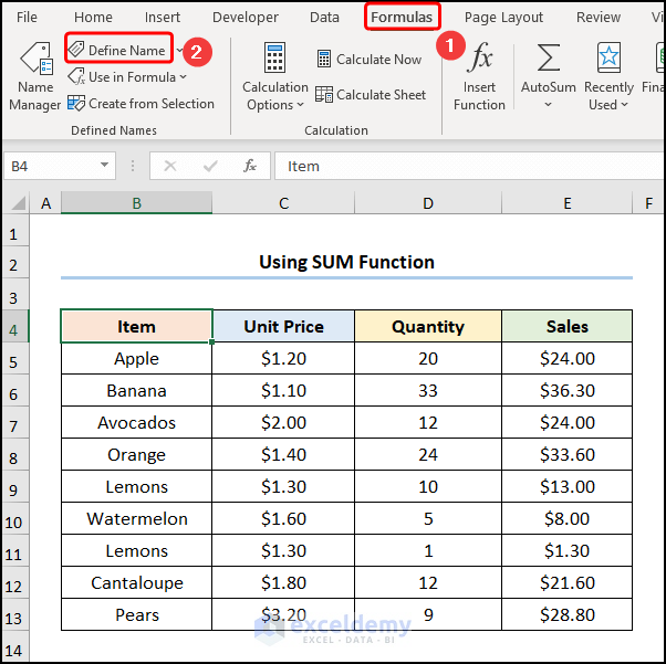
- Define a name (“Sales”) for E5:E13.
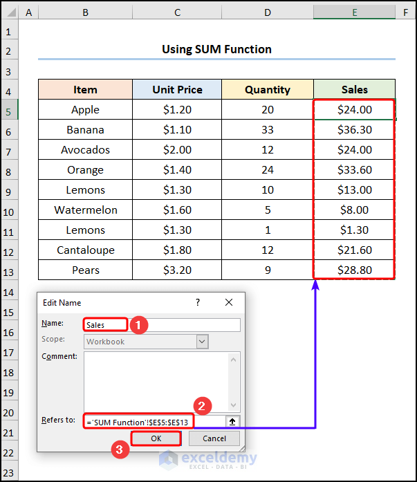
- Use the SUM function to obtain the “Total Sales” : “$190.60”.
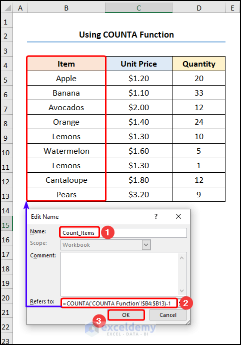
Example 3 – Utilizing the COUNTA Function
Steps:
- Follow the steps described in the Example 2 >> Choose a name. Here, “Count_Items” >> insert the formula below.
=COUNTA('COUNTA Function'!$B4:$B13)-1
The ‘COUNTA Function’!$B4:$B13) is the value argument that represents the B4:B13 in the “COUNTA Function”.
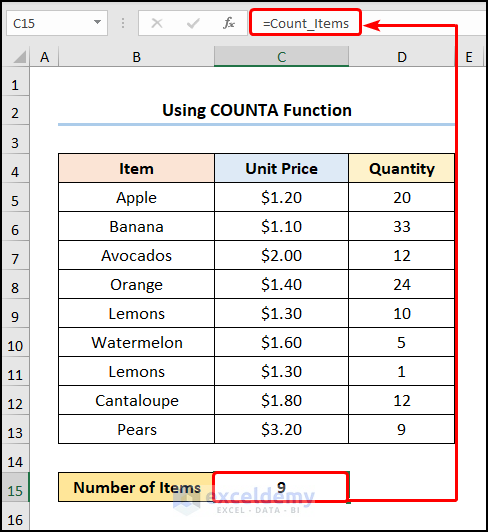
- Go to C15 >> enter the Defined Name “Count_Items” and press ENTER to see the count.
Note: You can open the list of Defined Names by pressing CTRL + F3.
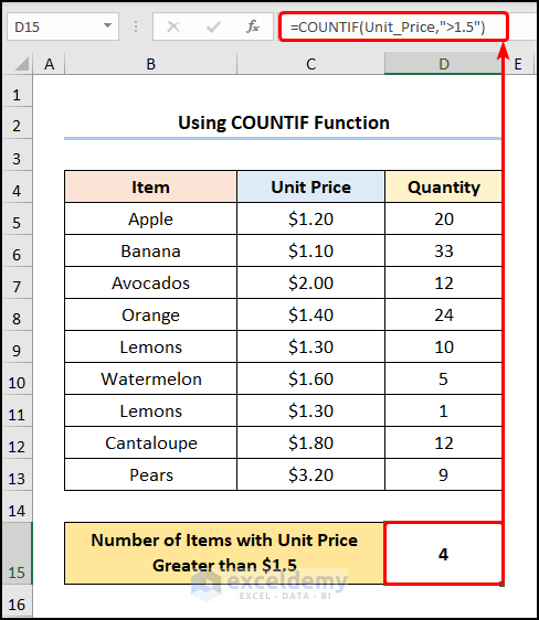
Example 4 -Using the COUNTIF Function
To count the number of items with a Unit Price” exceeding “$1.5”.
Steps:
- Go to D15 >> Enter the formula.
=COUNTIF(Unit_Price,">1.5")
The “Unit_Price” points to the Defined Name which indicates C5:C13.
Formula Breakdown:
- COUNTIF(Unit_Price,”>1.5″) → counts the number of cells within a range that meet the given condition. Here, Unit_Price represents the range argument that refers to C5:C13, whereas the “>1.5” indicates the criteria argument that returns the count of the values greater than “$1.50”.
- Output → 4
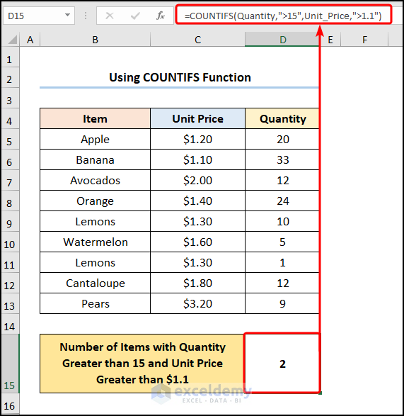
Example 5 – Applying the COUNTIFS Function
To see items in “Quantity” and “Unit Price” greater than “15” and “$1.1”.
Steps:
- Go to D15 >> Enter the formula in the Formula Bar.
=COUNTIFS(Quantity,">15",Unit_Price,">1.1")
“Quantity” and “Unit_Price” indicate the Defined Names.
Formula Breakdown:
- COUNTIFS(Quantity,”>15″,Unit_Price,”>1.1″) → counts the number of cells specified by a given set of conditions and criteria. Quantity represents the criteria_range1 argument that refers to D5:D13, whereas “>15” indicates the criteria1 argument that represents the condition greater than “15”. Unit_Price represents the criteria_range2 argument that refers to C5:C13, whereas “>1.1” indicates the criteria2 argument that represents the condition greater than “$1.1”.
- Output → 2
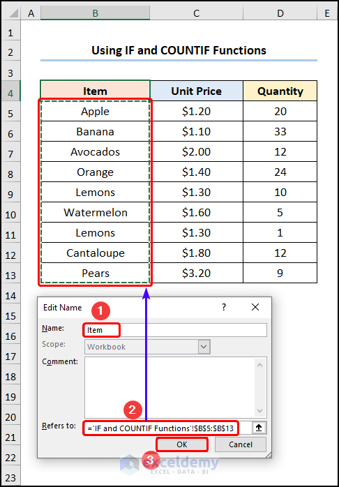
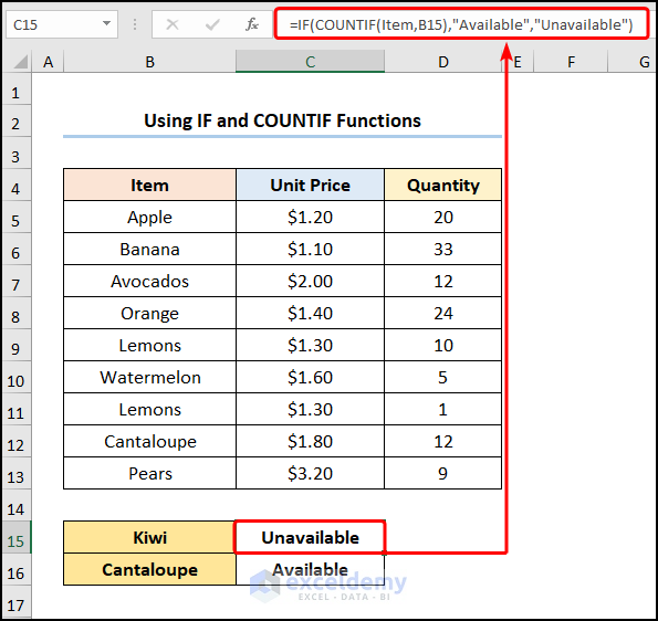
Example 6 – Combining the IF and the COUNTIF Functions
To check if the name of the fruit is in the list.
Steps:
- Follow the steps described in example 5 to create a Defined Name for “Item”.
- In C15, enter the formula below.
=IF(COUNTIF(Item,B15),"Available","Unavailable")
B15 cell indicates “Kiwi”.
Formula Breakdown:
- COUNTIF(Item,B15) → Item represents the range argument that refers to the Item column, whereas B15 indicates the criteria argument:“Kiwi”. Since “Kiwi” is not present, the function returns zero, which implies FALSE.
- Output → 0
- IF(COUNTIF(Item,B15),”Available”,”Unavailable”) → becomes
- IF(0,”Available”,”Unavailable”) → checks whether a condition is met and returns one value if TRUE and another value if FALSE. Here, 0 is the logical_test argument, which prompts the IF function to return “Unavailable” (value_if_false argument), otherwise, “Available” (value_if_true argument).
- Output → Unavailable
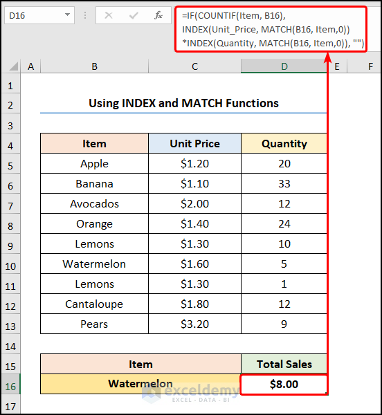
Example 7 – Using the INDEX and the MATCH Functions
To calculate the “Total Sales” based on a selected “Item”.
Steps:
- Go to D16 >> Enter the following formula
=IF(COUNTIF(Item, B16),INDEX(Unit_Price, MATCH(B16, Item,0))*INDEX(Quantity, MATCH(B16, Item,0)), "")
B16 refers to the “Watermelon”.
Formula Breakdown:
- MATCH(B16, Item,0) → returns the relative position of an item in an array matching the given value. B16 is the lookup_value argument that refers to “Watermelon”. Item represents the lookup_array argument from which the value is matched. 0 is the optional match_type argument which indicates Exact match criteria.
- Output → 6
- INDEX(Unit_Price, MATCH(B16, Item,0)) → becomes
- =INDEX(Unit_Price, 6) → returns a value at the intersection of a row and column in a given range. Unit_Price is the array argument. 6 is the row_num argument that indicates the row location.
- Output → $1.6
- IF(COUNTIF(Item, B16),INDEX(Unit_Price, MATCH(B16, Item,0))*INDEX(Quantity, MATCH(B16, Item,0)), “”) → becomes
- IF(1,1.6*5,””) → 1 is the logical_test argument which prompts the IF function to return 1.6*5 (value_if_true argument). Otherwise, it returns “” (Blank) (value_if_false argument).
- Output → $8.00
Read More: How to Create a Complex Formula in Excel
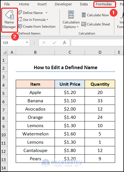
How to Edit a Defined Name in Excel
Steps:
- Go to the Formulas tab >> choose Name Manager.
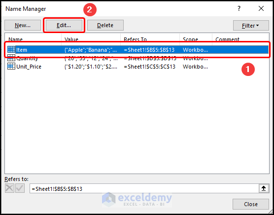
- Select a Defined Name, here “Item” >> Click Edit.
- Rename the range or enter a different range.
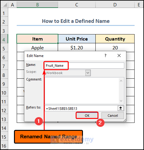
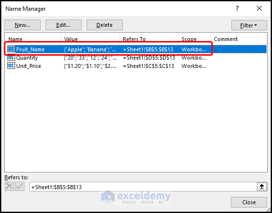
This is the output.
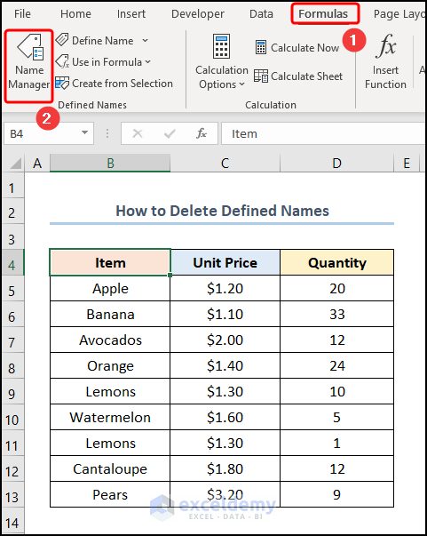
How to Delete Defined Names in Excel
Steps:
- Go to the Formulas tab >> select Name Manager.
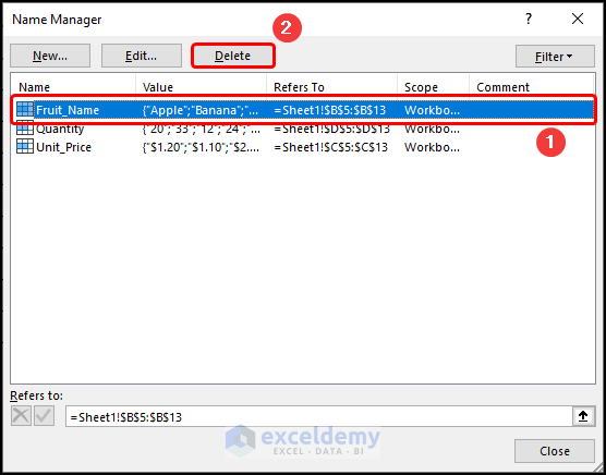
- Select the Defined Name. Here, “Fruit_Name” >> Click Delete.
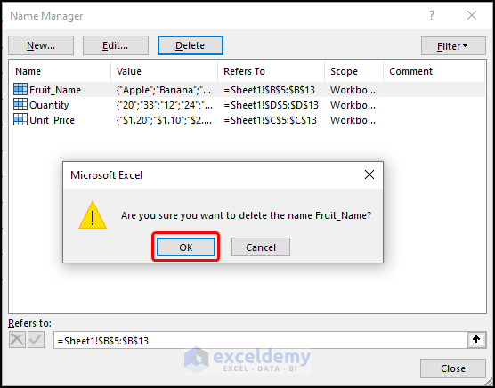
- Click OK to delete the Defined Name.
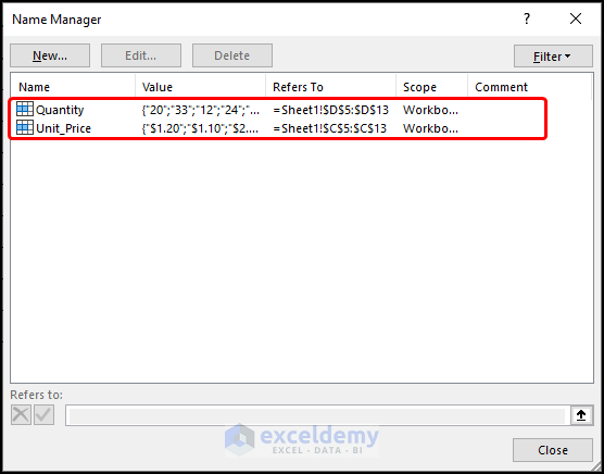
This is the output.
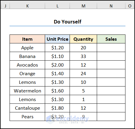
Practice Section
Practice here.
Download Practice Workbook
Related Articles
- How to Create a Formula in Excel for Multiple Cells
- How to Create a Custom Formula in Excel
- How to Apply Formula in Excel for Alternate Rows
- How to Insert Formula for Entire Column in Excel
- How to Create a Conditional Formula in Excel
<< Go Back to How to Create Excel Formulas | Excel Formulas | Learn Excel
Get FREE Advanced Excel Exercises with Solutions!
