How to Transpose Multiple Columns into One Column in Excel (3 Methods)

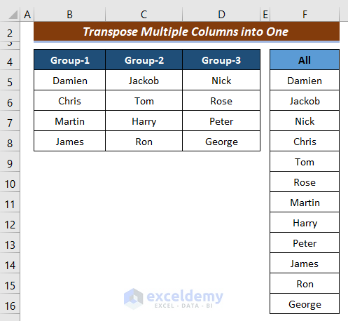
The following image highlights the purpose of this article.

Method 1 – Use Excel Formulas

1.1 Combine INDEX, INT, MOD, ROW, and COLUMNS Functions

• We’ll combine the INDEX, INT, MOD, ROW, and COLUMNS functions.
• Assume we have data in the range $B$5:$D$8 (you can adjust this range as needed).
• The goal is to create a one-column list from the transposed data.
• Follow these steps:

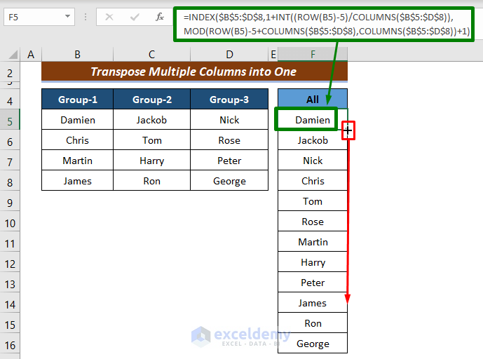
Step 1: Go to cell F5 (or any other empty cell where you want the transposed data) and enter the following formula:

Step 2: Press ENTER and then drag the fill handle icon down until the last entry appears in the one-column list.

 The screenshot below illustrates the procedure and the resulting transposed data:

Note:

• If your dataset starts from cell A1, replace ROW(5) – 5 with ROW(B5) – 5 with ROW(A1) – 1.
• The formula calculates the row and column numbers for the INDEX function.

Formula Explanation:

• The INDEX function has 3 arguments: array, row number, and column number.
• The array is $B$5:$D$8.
• The row number argument is calculated as follows:
  • 1 + INT((ROW(B5) – 5) / COLUMNS($B$5:$D$8))
  • This ensures that the row number starts from 1.

• The column number argument is calculated using:
  • MOD(ROW(B5) – 5 + COLUMNS($B$5:$D$8), COLUMNS($B$5:$D$8)) + 1
  • This determines the column position within the array.
• The result will be a single-column list with the transposed data.

1.2 Combine OFFSET, CEILING, MOD, ROW, and COLUMNS Functions

Generic Formula:

=OFFSET(Starting Cell’s absolute reference, CEILING((ROW(Starting cell reference)-m)/Number of columns,1), MOD(ROW(Starting cell reference)+Number of columns-n, Number of columns)

Where:

• m represents the starting cell’s row number plus 1 (if your dataset’s column number is even) or plus 2 (if your dataset’s column number is odd).
• n is a number that ensures the result of (ROW(Starting cell reference) + Number of columns – n) is completely divisible by the number of columns.

Step-by-Step Procedure:

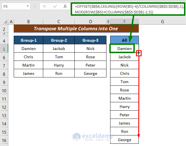
• Copy the following formula and paste it into cell F5:

• Press ENTER.
• Drag the Fill Handle icon all the way down.

The screenshot below illustrates the process:

Formula Explanation:

• The OFFSET function has 3 compulsory arguments: reference, rows, and columns.
• $B$4 serves as the reference for the OFFSET function, indicating where the offsetting should start.
• The CEILING((ROW(B5)-4)/COLUMNS($B$5:$D$8),1) part determines the rows argument:
  • It ensures that the row number starts from 1.
• The MOD(ROW($B5)+COLUMNS($B$5:$D$8)-2,3) part determines the columns argument:
  • It calculates the column position within the array.
• The result will be the value in the transposed position, which in this case is “Damien.”

1.3 Combine OFFSET, ROUNDUP, MOD, and ROWS Functions

Generic Formula:

=OFFSET(Absolute Ref. of the cell situated just above the starting cell, ROUNDUP((ROWS($X:X))/Number of columns, 0), MOD(ROWS($X:X)+n, Number of columns)

Where,

X= represents the starting row of the dataset (not the heading).

n= s a number that ensures the output of ROWS($X:X)+n is completely divisible by the number of columns in your dataset.

Step-by-Step Procedure:

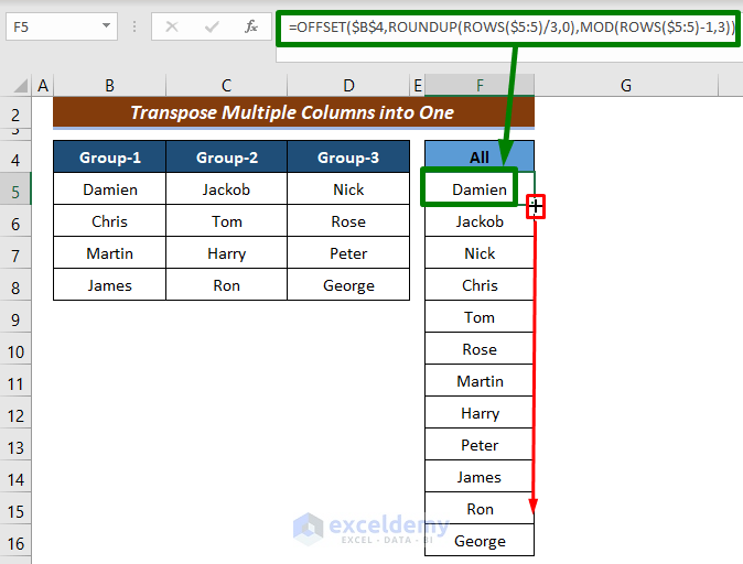
• Insert the following formula into cell F5 and press ENTER:

=OFFSET($B$4,ROUNDUP(ROWS($5:5)/3,0),MOD(ROWS($5:5)-1,3))

• Drag the Fill Handle icon all the way down.

The screenshot below illustrates the process:

Formula Explanation:

• The OFFSET function has three compulsory arguments: reference, rows, and columns.
• $B$4 serves as the reference for the OFFSET function, indicating where the offsetting should start (just above the starting cell).
• The ROUNDUP(ROWS($5:5) /3, 0) part determines the rows argument:
  • It ensures that the row number starts from 1.
• The MOD(ROWS($5:5) – 1, 3) part determines the columns argument:
  • It calculates the column position within the array.
• The result will be the value in the transposed position.

Similar Readings

• How to Transpose Rows to Columns Based on Criteria in Excel
• How to Transpose Rows to Columns Using Excel VBA (4 Ideal Examples)
• How to Transpose Rows to Columns in Excel (5 Useful Methods)
• How to Transpose Columns to Rows In Excel (6 Methods)

Method 2 – Use an Excel VBA Code

• Press Alt+F11:
  • This opens the Visual Basic for Applications (VBA) editor.
• Go to the Insert tab and select Module:
  • This action creates a new VBA module where we’ll insert our code.

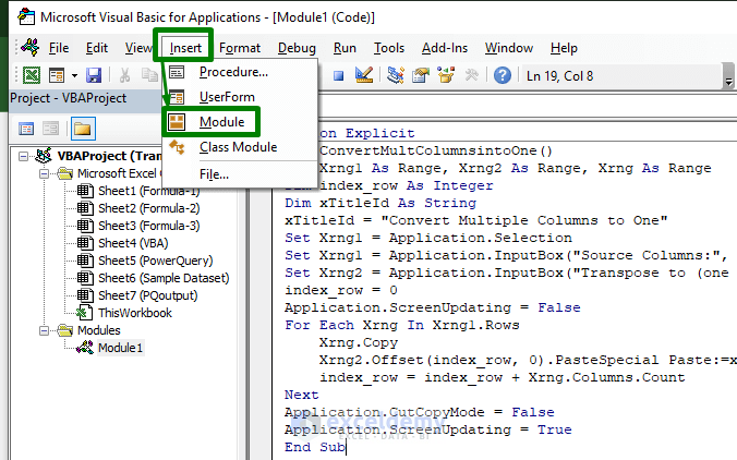
• Copy and paste the following VBA code into the opened module:

Option Explicit
Sub ConvertMultColumnsintoOne()
Dim Xrng1 As Range, Xrng2 As Range, Xrng As Range
Dim index_row As Integer
Dim xTitleId As String
xTitleId = "Convert Multiple Columns to One"
Set Xrng1 = Application.Selection
Set Xrng1 = Application.InputBox("Source Columns:", xTitleId, Xrng1.Address, Type:=8)
Set Xrng2 = Application.InputBox("Transpose to (one column):", xTitleId, Type:=8)
index_row = 0
Application.ScreenUpdating = False
For Each Xrng In Xrng1.Rows
    Xrng.Copy
    Xrng2.Offset(index_row, 0).PasteSpecial Paste:=xlPasteAll, Transpose:=True
    index_row = index_row + Xrng.Columns.Count
Next
Application.CutCopyMode = False
Application.ScreenUpdating = True
End Sub

• Press the F5 key to run the code:
  • This executes the VBA macro.
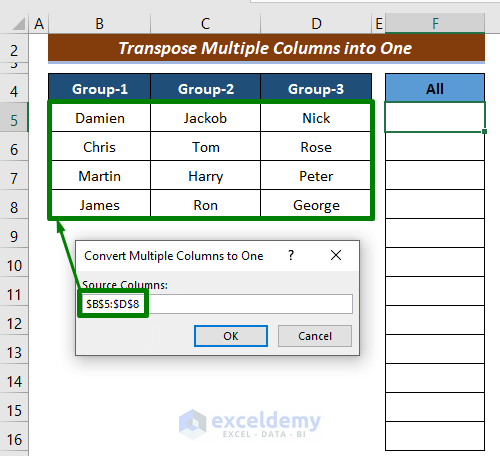
• Select the Source Columns (e.g., B5:D8):
  • When prompted, choose the range of columns you want to transpose.
• Press OK.

• Select the destination cell (e.g., F5) where you want to place the transposed data.

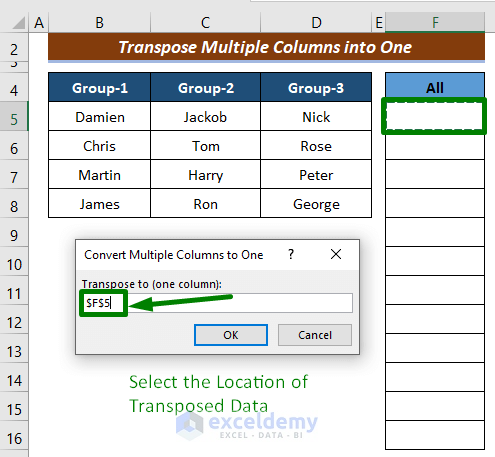
You will see the results like this:

The VBA code copies data from the source columns and pastes it transposed into the specified destination cell.

Read More: VBA to Transpose Multiple Columns into Rows in Excel (2 Methods)

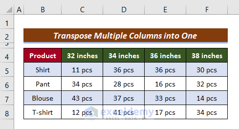
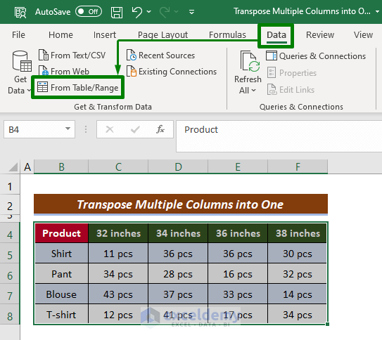
Method 3 – Use the Power Query Tool

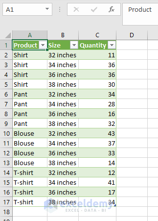
In this section of the article, we’ll be working with a dataset that differs from the one we’ve used so far. Our dataset contains product names, sizes, and quantities in separate columns. Our goal is to consolidate this information into single columns for product, size, and quantity. To achieve this, we’ll utilize the Power Query tool.

Follow these steps:

• Select either the entire dataset or any specific cell within it.
• Navigate to the Data tab in Excel.
• Click the From Table/Range button located in the Get & Transform Data group.

• The Create Table window will appear.

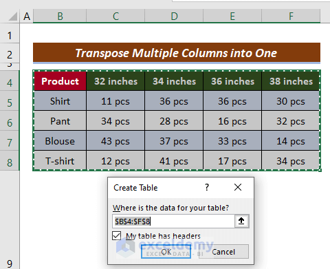
• Check the My table has headers checkbox.
• Click OK.
• The Power Query Editor window will open.
• Go to the Transform tab.
• Select the first column of your data.
• Click the drop-down menu for Unpivot Columns in the Any Column group.
• Choose the Unpivot Other Columns option.

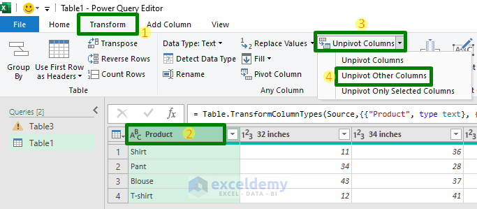
You will see the following:

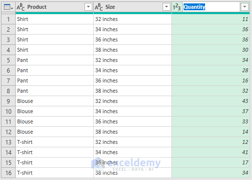
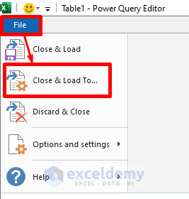
• Switch to the File tab.
• Click the Close & Load To… button.

• A window will appear.
• Select your preferred location (existing or new worksheet).

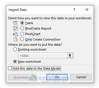
• Click OK.

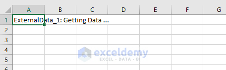
Your results will be displayed. Since you’ve chosen the New Worksheet option, the results will appear on a new sheet.

Read More: Excel Power Query: Transpose Rows to Columns (Step-by-Step Guide)

Things to Remember

• Adjust Formulas for Dataset Size:
  • When working with your dataset, make sure to modify the formulas based on its size. Different datasets may require different approaches.
• #REF! Error or Starting with 0:
  • If you encounter a #REF! error or if your results start with 0, it could indicate that you’ve inadvertently combined all the entries into a single column. Double-check your calculations and ensure that you’re handling the data correctly.

Related Articles

• • • How to Transpose Duplicate Rows to Columns in Excel (4 Ways)
    • How to Transpose Every n Rows to Columns in Excel (2 Easy Methods)
    • Excel VBA: Transpose Multiple Rows in Group to Columns
    • Convert Columns to Rows in Excel Using Power Query
    • How to Convert Columns to Rows in Excel Based On Cell Value
    • VBA to Transpose Multiple Columns into Rows in Excel (2 Methods)
    • How to Convert Column to Comma Separated List With Single Quotes

Download Practice Workbook

You can download the practice workbook from here:

Transpose Multiple Columns into One.xlsm