Download the Practice Workbook
2 Handy Approaches to Transpose Rows to Columns Based on Criteria in Excel
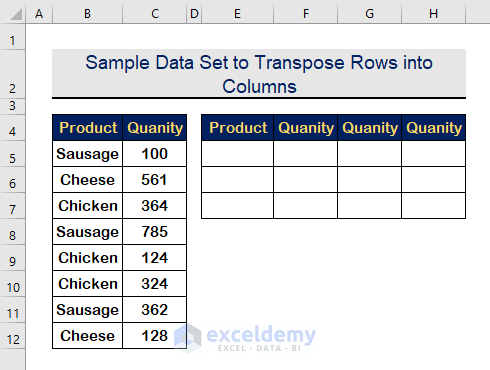
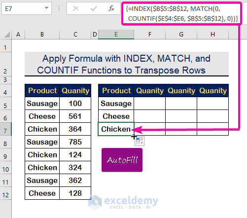
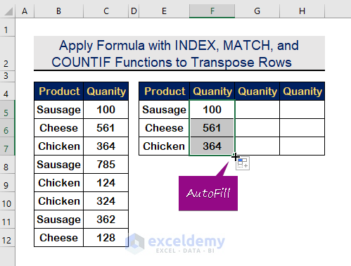
We’ve included a data set of several products and their quantities in the figure below. The rows will then be transposed into columns. We’ll transpose the rows into columns based on the criteria of the unique values because there are some duplicate entries in a separate cell.
Method 1 – Apply a Formula with the INDEX, MATCH, and COUNTIF Functions to Transpose Rows to Columns Based on Criteria in Excel
Steps
- In cell E5, use the following formula to get the unique products.
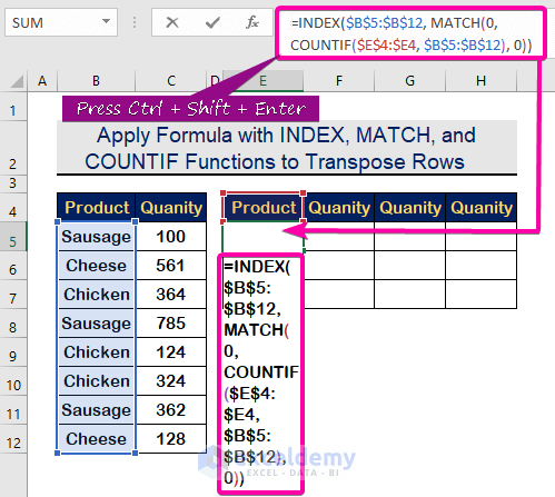
=INDEX($B$5:$B$12, MATCH(0, COUNTIF($E$4:$E4, $B$5:$B$12), 0))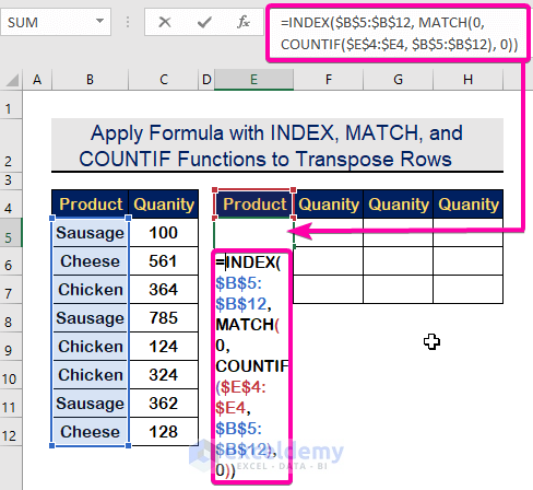
- To apply the formula with an array in versions of Excel that are not Excel 365, press Ctrl + Shift + Enter.
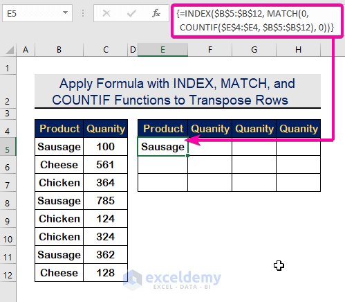
- You will get the first unique result.
- To get all the unique values, use the AutoFill Handle Tool to auto-fill the column.
- To transpose the row value of quantities into columns, use the following formula.
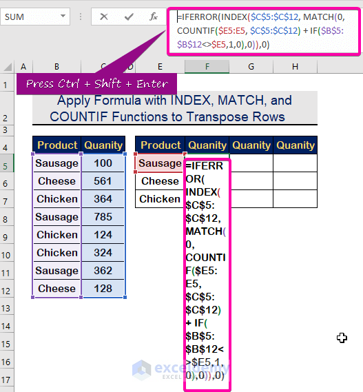
=IFERROR(INDEX($C$5:$C$12, MATCH(0, COUNTIF($E5:E5, $C$5:$C$12) + IF($B$5:$B$12<>$E5,1,0),0)),0)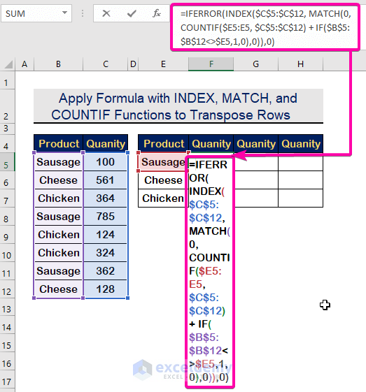
- To apply the formula with an array in versions of Excel that are not Excel 365, press Ctrl + Shift + Enter.
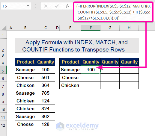
- The cell F5 will show the first transposed value as in the image shown below.
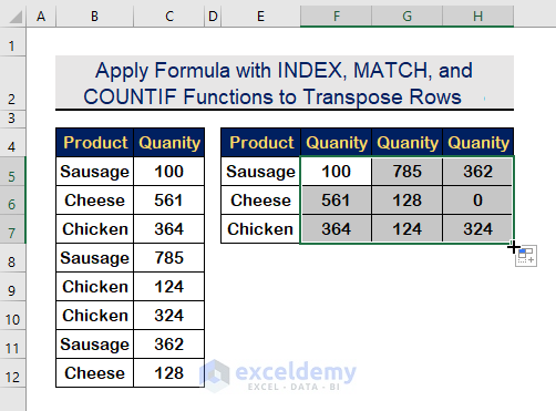
- Drag down with the AutoFill Handle Tool to auto-fill the column.
- Auto-fill the rows with the AutoFill Handle Tool.
Similar Readings
- How to Transpose Duplicate Rows to Columns in Excel (4 Ways)
- Transpose Multiple Columns into One Column in Excel (3 Handy Methods)
- How to Reverse Transpose in Excel (3 Simple Methods)
Method 2 – Run a VBA Code to Transpose Rows to Columns Based on Criteria in Excel
Steps
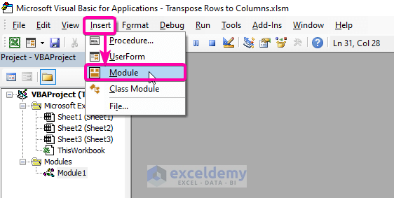
- Press Alt + F11 to open the VBA window.
- Click on Insert.
- Select the Module option.
- Paste the following VBA code into the module:
Sub TransposeRows()
'Define Variables
    Dim RowsNumber As Long
    Dim p As Long
    Dim xColCr As String
    Dim xColumn  As New Collection
    Dim InputRng As Range
    Dim OutputRng As Range
    Dim RngText As String
    Dim CountRow As Long
    Dim xRowRg As Range
    On Error Resume Next
'Set values and Input Box fot Input Range
    RngText = ActiveWindow.RangeSelection.Address
    Set InputRng = Application.InputBox("Select Your Input Range for 2 columns:", "ExcelDemy", RngText, , , , , 8)
    Set InputRng = Application.Intersect(InputRng, InputRng.Worksheet.UsedRange)
'Apply Condition to count only 2 columns and to show msg box for alerting to select only two columns
    If InputRng Is Nothing Then Exit Sub
    If (InputRng.Columns.Count <> 2) Or _
       (InputRng.Areas.Count > 1) Then
        MsgBox "The specified range is only area for 2 columns ", , "ExcelDemy"
        Exit Sub
    End If
'Set values and Input Box fot Input Range
    Set OutputRng = Application.InputBox("Select Your Output Range (one cell):", "ExcelDemy", RngText, , , , , 8)
    If OutputRng Is Nothing Then Exit Sub
    Set OutputRng = OutputRng.Range(1)
'Count Rows
    RowsNumber = InputRng.Rows.Count
'Apply For loop
    For p = 2 To RowsNumber
        xColumn.Add InputRng.Cells(p, 1).Value, InputRng.Cells(p, 1).Value
    Next
    Application.ScreenUpdating = False
    For p = 1 To xColumn.Count
        xColCr = xColumn.Item(p)
        OutputRng.Offset(p, 0) = xColCr
        InputRng.AutoFilter Field:=1, Criteria1:=xColCr
        Set xRowRg = InputRng.Range("B2:B" & RowsNumber).SpecialCells(xlCellTypeVisible)
        If xRowRg.Count > CountRow Then CountRow = xRowRg.Count
'Copy and paste with transpose
        InputRng.Range("B2:B" & RowsNumber).SpecialCells(xlCellTypeVisible).Copy
        OutputRng.Offset(p, 1).PasteSpecial Paste:=xlPasteAll, Operation:=xlNone, SkipBlanks:=False, Transpose:=True
        Application.CutCopyMode = False
    Next
    OutputRng = InputRng.Cells(1, 1)
    OutputRng.Offset(0, 1).Resize(1, CountRow) = InputRng.Cells(1, 2)
    InputRng.Rows(1).Copy
    OutputRng.Resize(1, CountRow + 1).PasteSpecial Paste:=xlPasteFormats
    InputRng.AutoFilter
    Application.ScreenUpdating = True
End Sub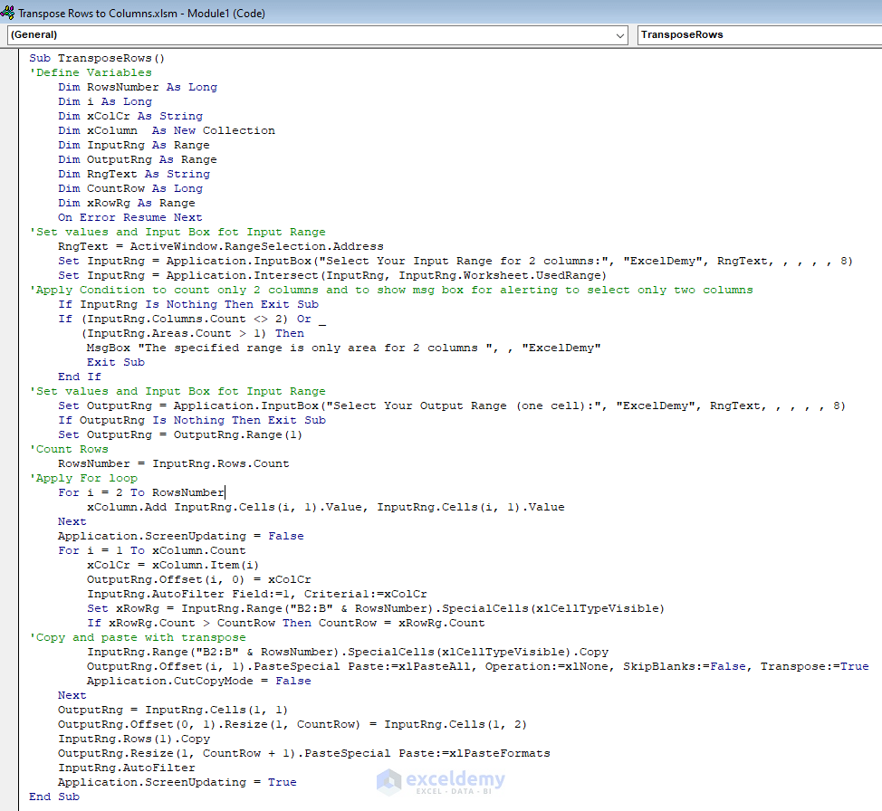
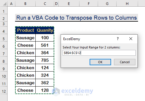
- Save and press F5 to run the program.
- Select your data set with the header.
- Click on OK.
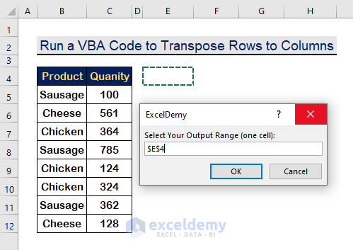
- Select a cell to get the output
- Click on OK.
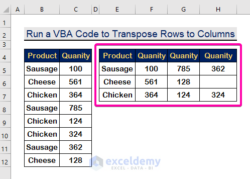
- Here’s the result.
Read More: How to Transpose Rows to Columns Using Excel VBA (4 Ideal Examples)
Related Articles
- Convert Columns to Rows in Excel Using Power Query
- How to Convert Columns to Rows in Excel Based On Cell Value
- VBA to Transpose Multiple Columns into Rows in Excel (2 Methods)
- How to Convert Column to Comma Separated List With Single Quotes
- Excel Paste Transpose Shortcut: 4 Easy Ways to Use
- Excel Transpose Formulas Without Changing References (4 Easy Ways)
- How to Transpose in Excel VBA (3 Methods)


The VBA code is not working. Tried several times.
Greetings UNSOLVABLE,
We have just rechecked our code and it is working. You might have any compatibility issues for not working this code. You may download our sample Excel file and try to apply the code on that.
Alternatively, you can share your Excel file on our forum https://exceldemy.com/forum/. We will solve your issues within no time.
Best Regards,
Bhubon Costa, Exceldemy