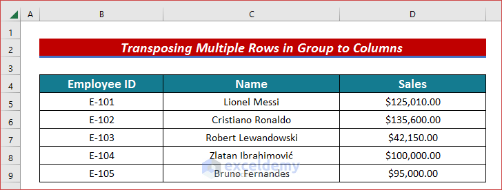
Microsft Excel has made data collection very easy. It has lots of functions and formulas that can be used as per our need. Here we will discuss how to transpose multiple rows in the group to columns in Excel. Manually transposing is very stressful work. In this article, I will try to explain 5 suitable ways to transpose multiple rows in group to columns in Excel. I hope it will be very helpful for you if you are looking for an efficient way to do so.
Download Practice Workbook
Download this practice sheet to exercise while you are reading this article.
5 Suitable Ways to Transpose Multiple Rows in Group to Columns in Excel
In order to transpose rows into columns, we will describe 5 suitable ways to do so. We can use Paste Special command, the TRANSPOSE, INDIRECT, INDEX functions, and the Form Table features. To clarify the methods, I have used the dataset with sales records in the Employee ID, Name, and Sales columns.
1. Use Paste Special Feature to Transpose Multiple Rows in Group to Columns
The easiest way to transpose rows to columns is by using the Paste Special feature. You can implement this Paste Special with both Ribbon Commands and Keyboard shortcuts.
1.1 Use Paste Special Feature from Ribbon
First, we will discuss the Paste Special feature from Ribbon.
Steps:
- Select the range (i.e. B4:D9) that you want to transpose.
- Then fro your Home tab, go to,
Home → Clipboard → Copy
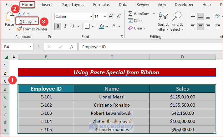
- After that, select the cell where you want to transpose (i.e. B12).
- From the ribbon, go to the Paste drop-down and select Transpose(T).
![]()
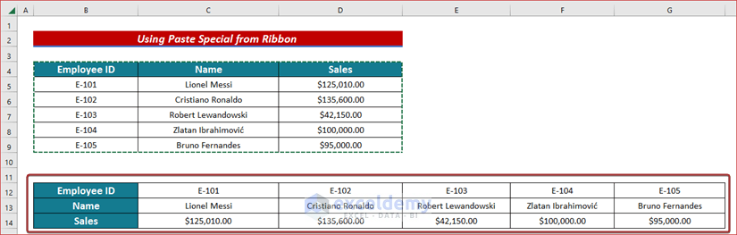
- Thus, we can simply transpose rows to columns by using the Paste Special feature.
1.2 Utilize Keyboard Shortcut
We can also do the similar task by using Keyboard Shortcut. Let’s march forward.
Steps:
- First, select the entire range (i.e. B4:D9) you want to tanspose.
- Press Ctrl + C .

- After that, select the cell where you will transpose.
- Press Ctrl + V .
![]()
- After that from the drop-down, select Transpose marked as red.
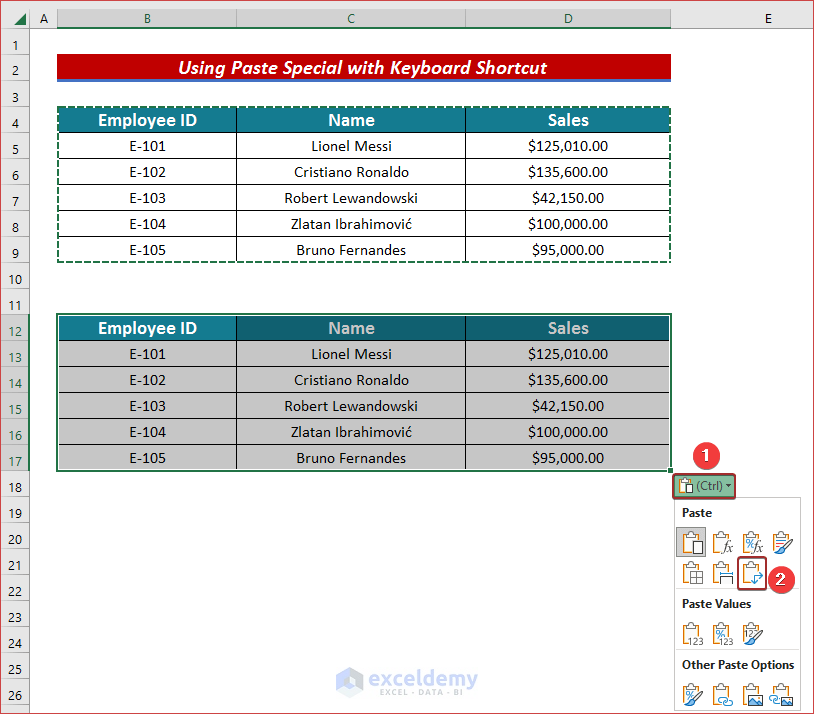
- Finally, you will get the desired transposed result.
![]()
Read More: Excel Paste Transpose Shortcut: 4 Easy Ways to Use
2. Apply TRANSPOSE Function to Transpose Multiple Rows in Group to Columns
Excel has a default function to transpose, which is TRANSPOSE. You can transpose easily by using this function. You need to use function keys for this function.
Steps:
- Select a cell first (i.e. B12).
- Now, insert the following formula in that cell to have transposed output.
=TRANSPOSE(B4:D9)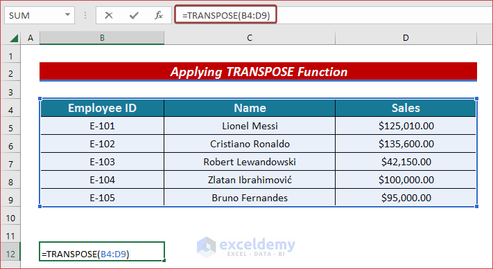
- Press the ENTER button to have the result.
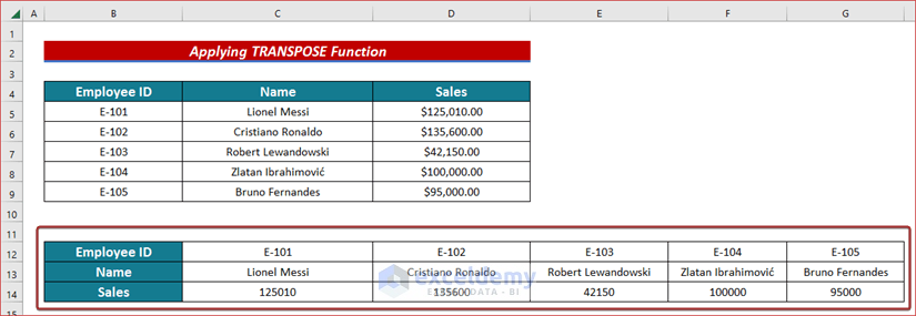
![]()
- You can modify the transposed results according to your choice.
Read More: How to Transpose Rows to Columns Using Excel VBA (4 Ideal Examples)
Similar Readings
- How to Transpose Duplicate Rows to Columns in Excel (4 Ways)
- How to Convert Columns to Rows in Excel (2 Methods)
- Transpose Multiple Columns into One Column in Excel (3 Handy Methods)
- How to Reverse Transpose in Excel (3 Simple Methods)
- How to Convert Multiple Columns into a Single Row in Excel (2 Ways)
3. Transpose Multiple Rows in Group to Columns with INDIRECT Function
The INDIRECT function is another function that can be used to transpose multiple rows in group to columns. The whole process is described in the following section.
Steps:
- Write the following formula in your preferred location and press ENTER to have the first value of your transposed data.
.
=INDIRECT(ADDRESS(COLUMN(B4) - COLUMN($B$4) + ROW($B$4), ROW(B4) - ROW($B$4) + COLUMN($B$4)))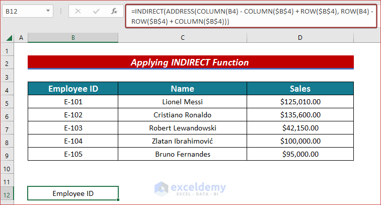
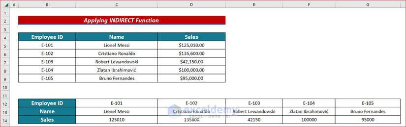
- Now, use AutoFill Handle across the horizontal line to have automatically filled transposed data.
![]()
- Next, move the AutoFill Handle across the vertical line to have the entire transposed data.
![]()
- Now, modify the transposed results according to your choice.
Read More: Excel Transpose Formulas Without Changing References (4 Easy Ways)
4. Utilize INDEX Function to Transpose Multiple Rows in Group to Columns
Using the INDEX function, we can easily understand how to tackle the data which is arranged in rows to shift in columns. To understand the process in detail, go through the following steps.
Steps:
- Insert the following formula in your preferred location and press ENTER to have the first value of your transposed data.
=INDEX($B$4:$D$9,COLUMN()-1,1)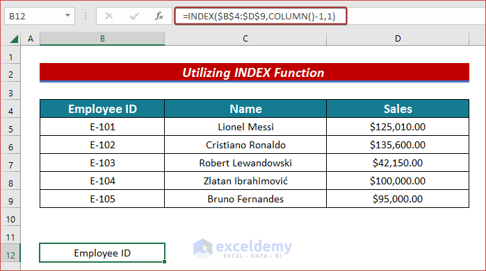
- To have automatically filled transposed data, use AutoFill Handle across the horizontal line.
![]()
- Similarly, input the following formula and drag along horizontally to have transposed data for the rest of the rows.
=INDEX($B$4:$D$9,COLUMN()-1,3)
Read More: How to Transpose Array in Excel (3 Simple Ways)
5. Transpose Multiple Rows in Group to Columns Using Form Table Feature
Another simple yet smart way to transpose multiple rows to columns is to use the Form Table feature. Follow the following procedures to execute the purpose.
Steps:
- First, select the range you want to transpose.
- Then, go to Data.
- After that, click From Table from the ribbon.
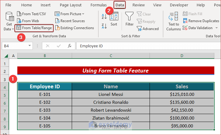
- We will see a POP UP that shows the range we selected.
- We can also change the range and check My table has headers as our table has headers.
- Then click OK.
![]()
- Now, we will see a new window named Powe Query Editor.
- Followingly, select all the columns.
- Next, go to Transform.
- Then, click Transpose from the ribbon.
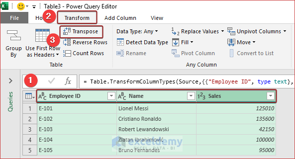
- Now, we will have the entire data transposed.
![]()
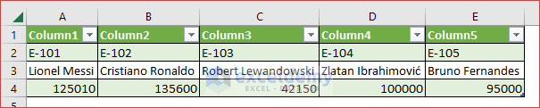
- Close the Powe Query Editor and we will have the transposed data in a new sheet.
Read More: Conditional Transpose in Excel (2 Examples)
Conclusion
At the end of this article, I like to add that I have tried to explain 5 suitable ways to transpose multiple rows in group to columns in Excel. It will be a matter of great pleasure for me if this article could help any Excel user even a little. For any further queries, comment below. You can visit our site for more articles about using Excel.
Further Readings
- Data clean-up techniques in Excel: Changing vertical data to horizontal data
- How to Swap Rows in Excel (2 Methods)
- Convert Columns to Rows in Excel (2 Methods)
- Excel VBA: Transpose Multiple Rows in Group to Columns
- How to Transpose Every n Rows to Columns in Excel (2 Easy Methods)
- VBA to Transpose Multiple Columns into Rows in Excel (2 Methods)
- Transpose Multiple Rows in Group to Columns in Excel

