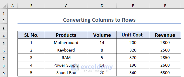
We’ll use a sample dataset with five columns: Serial No., Products, Volume, Unit Cost, and Revenue to illustrate how to take data arranged in columns and present it in rows within Excel.
Method 1 – Transposing Data to Convert Columns to Rows
The data shows Sales by Month in different countries. Now, we will be transposing the columns to rows.
1.1. Using the Context Menu Bar
We will use the Paste Options from the Context Menu Bar to convert columns to rows. Here are the steps:
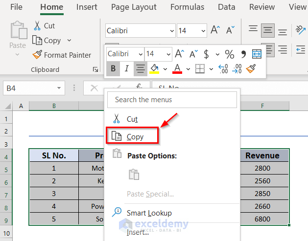
- Select the whole dataset.
- Right-Click on the dataset and the Context Menu Bar will open.
- Click on the Copy button (you can also select the dataset and then press CTRL+C)
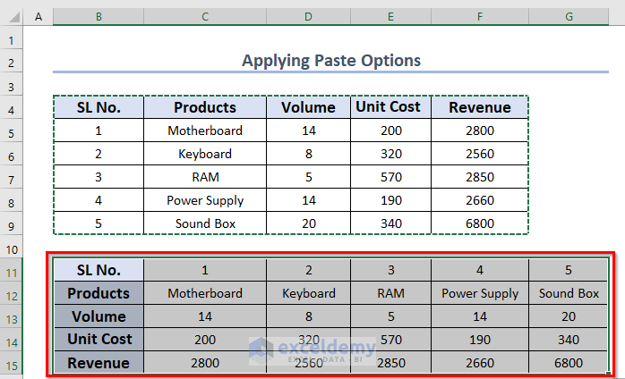
As a result, the dataset will be highlighted.
- Select the B11 cell for your output.
- Right-Click on the cell, and under Paste Options, choose Transpose (T).
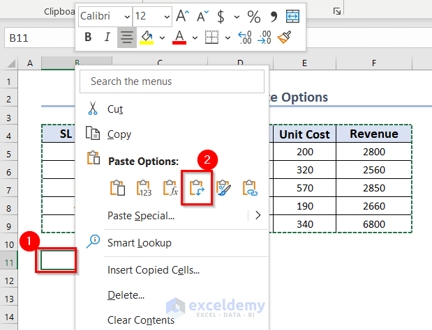
You will see the following image.
Read More: VBA to Transpose Multiple Columns into Rows in Excel
1.2. Applying Paste Special Feature
Steps:
- Select the whole dataset.
- Under Home, click on the Copy command found under the Clipboard group of commands.
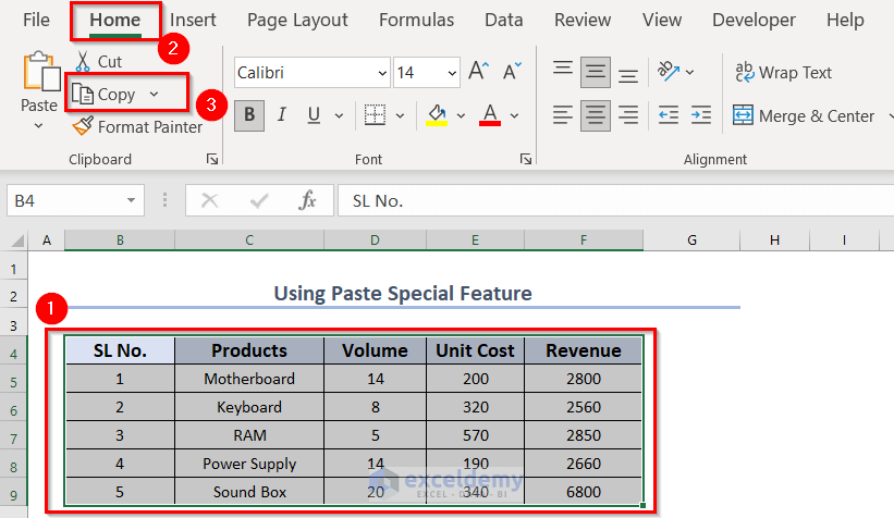
You’ve now copied the dataset.
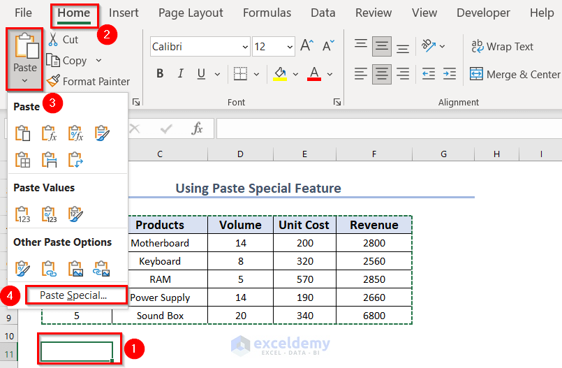
- Select the B11 cell for your output.
- Under the Home tab, click on Paste.
- Choose Paste Special option.
- Mark Transpose.
- After that, press OK.
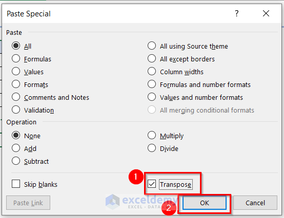
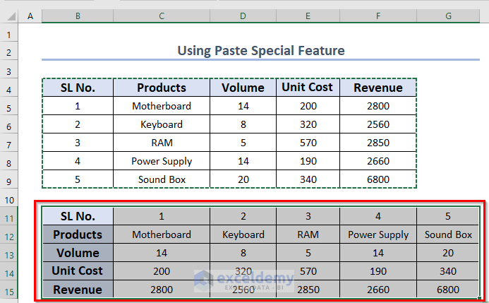
You will see the converted rows.
Read More: Convert Columns to Rows in Excel Using Power Query
Method 2 – Using INDIRECT & ADDRESS Functions in Excel
This method uses INDIRECT, ADDRESS, COLUMN, and ROW functions.
Steps:
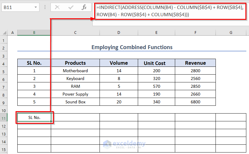
- Select a cell where you want the result. We have selected the B11 cell.
- Use the corresponding formula in the B11 cell:
=INDIRECT(ADDRESS(COLUMN(B4) - COLUMN($B$4) + ROW($B$4), ROW(B4) - ROW($B$4) + COLUMN($B$4)))- Press ENTER.
Formula Breakdown
- COLUMN(B4)—> returns the column number from a given reference.
- Output: {2}.
- ROW(B4)—> returns the row number from a given reference.
- Output: {4}.
- ROW(B4) – ROW($B$4) + COLUMN($B$4)—> becomes {4}-{4}+{2}. Here, the Dollar Sign ($) will fix column B.
- Output: {2}.
- COLUMN(B4) – COLUMN($B$4) + ROW($B$4)—> becomes {2}-{2}+{4}. Here, the Dollar Sign ($) will fix column B.
- Output: {4}.
- The ADDRESS function will return the position of row number 4 and column number 2.
- Output: {“$B$4”}.
- The INDIRECT function will return the value of that cell.
- Output: SL No.
- Drag the Fill Handle icon to AutoFill the corresponding data in cells B12:B15.
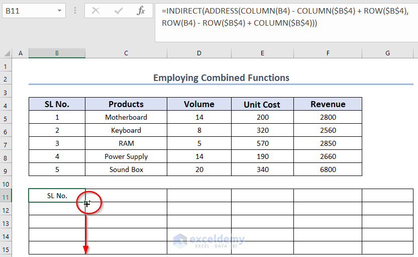
- Additionally, drag the Fill Handle icon to AutoFill the corresponding data in cells C12:G15.

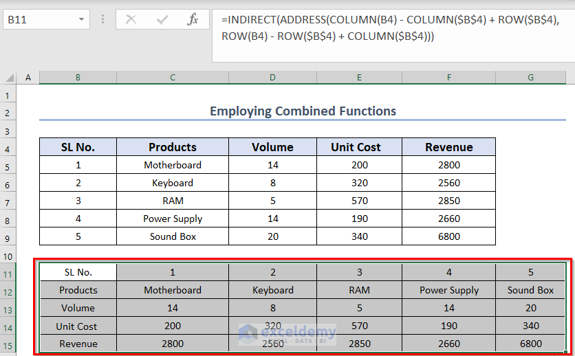
You will see the converted rows.
Read More: How to Transpose Duplicate Rows to Columns in Excel
Method 3 – Using TRANSPOSE Function to Convert Columns to Rows
Sometimes you may want to rotate cells. While the methods mentioned above can help you rotate data, they might introduce duplicate values. As an alternative approach, we will use a formula that leverages the TRANSPOSE function. We’ll revisit the same dataset we used previously to demonstrate this method.
Steps:
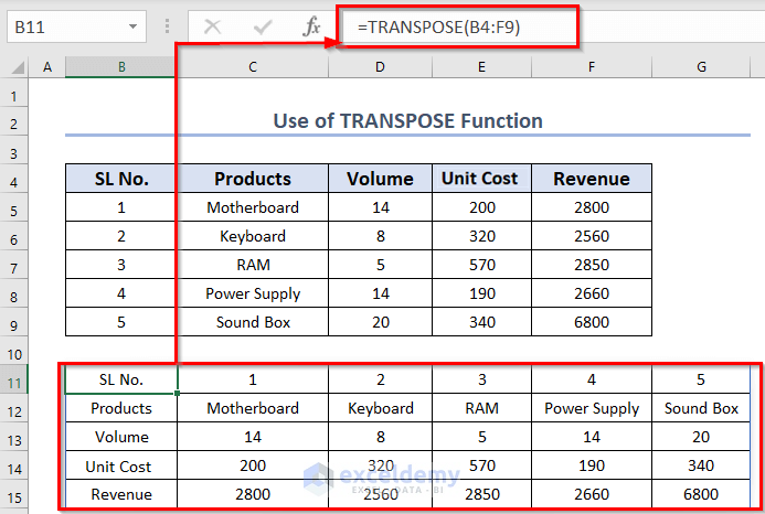
- Select a blank cell. (we selected B11). Count the number of cells in B4:F9. In this case, it is 30 cells.
- Type the range of the cells you want to transpose. In our example, we want to transpose cells from B4 to F9. So the formula would be:
=TRANSPOSE(B4:F9)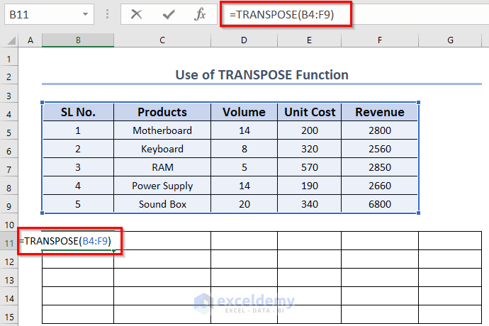
- Press ENTER.
The formula will be applied to more than one cell. Here’s the result:
Read More: How to Convert Multiple Columns into a Single Row in Excel
How to Solve TRANSPOSE Function & SPILL Errors in Excel
The Transpose function is bound to the original data. For example, if we change the value in D5 from 14 to 2, the new value will automatically be updated. But the reverse isn’t true.
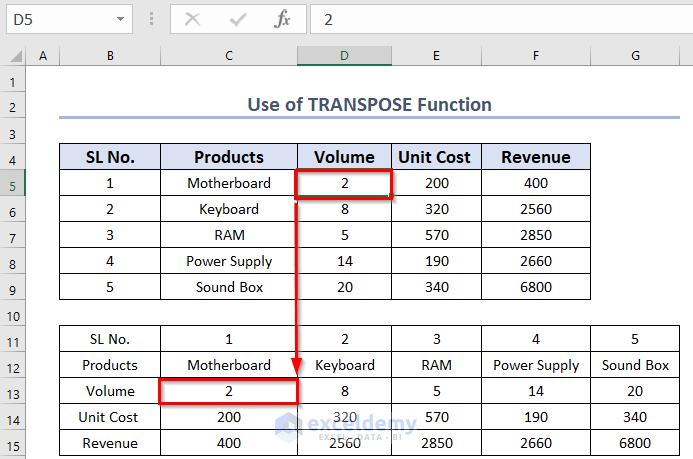
If we change any transposed cells, the original set will not change. Instead, we will get a SPILL error and the transposed data will disappear.

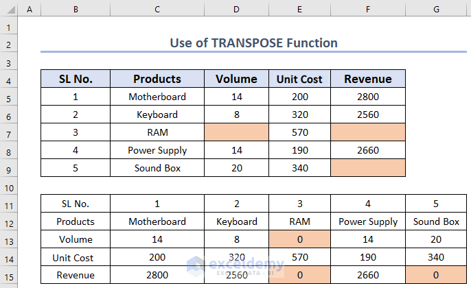
How to Use TRANSPOSE Function with Blank Cells in Excel
The TRANSPOSE function will convert the empty cells to “0”s. Check the image below:
Read More: How to Transpose Formulas Without Changing References in Excel
How to Convert Rows to Columns in Excel
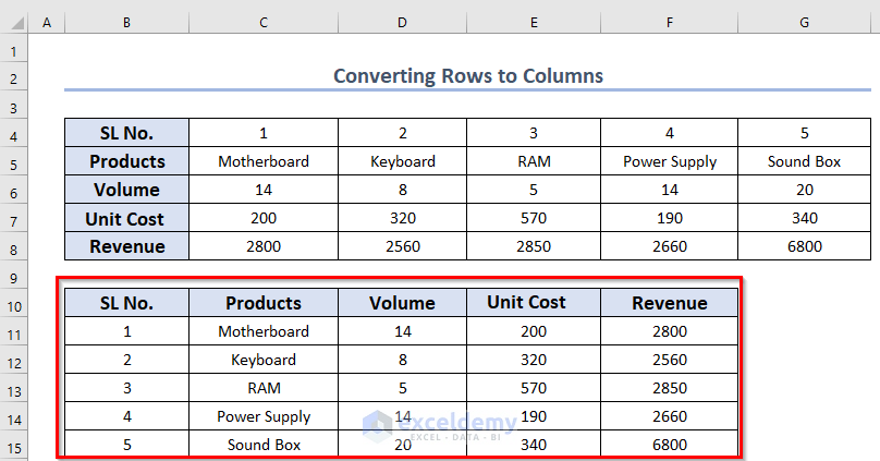
Let’s take the following dataset, where information is organized in rows, and transform the data into a columnar format.
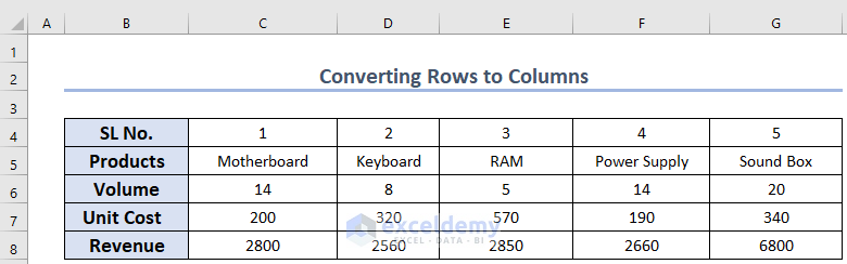
You can follow method-1 to convert the rows to columns. Actually, you can follow any of the methods but the method 1 is the easiest.
After following the steps, you will get the following coverted dataset:
Read More: How to Transpose Every n Rows to Columns in Excel
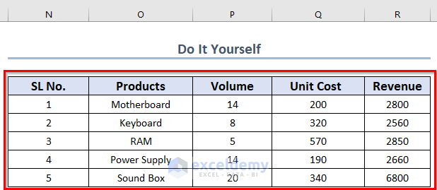
Practice Section
Practice the explained methods by yourself using the following dataset:
Download practice workbook
You can download the Practice Workbook we used for this article.
Further Readings
- How to Transpose Every n Rows to Columns in Excel
- How to Change Vertical Column to Horizontal in Excel
- Excel Power Query: Transpose Rows to Columns
- Excel VBA to Transpose Array
- How to Swap Rows in Excel

