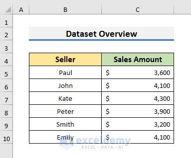
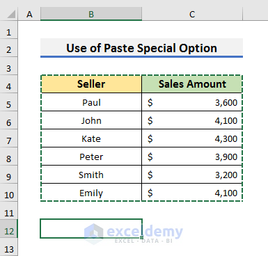
This is the sample dataset.
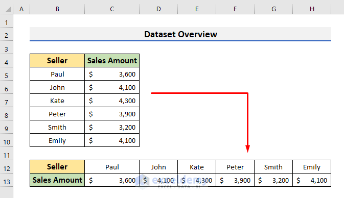
This will be the output:
Method 1 – Change a Vertical Column to a Horizontal row using the Paste Special Option in Excel
- Select B4:C10.
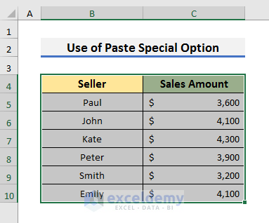
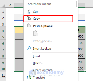
- Right-click.
- Select Copy. You can also press Ctrl + C to copy the range.
- Select a cell to paste the range horizontally. Here, B12.
- Go to the Home tab and click Paste.
- Select Paste Special. You can also press Ctrl + Alt + V to open the Paste Special box.
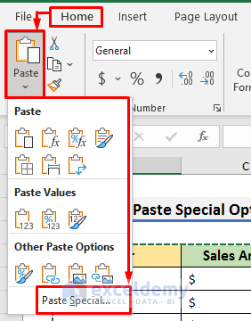
- Check Transpose and click OK.

This is the output.
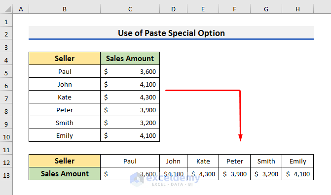
Note: The horizontal rows will not update dynamically.
Method 2 – Using the Excel TRANSPOSE Function to Convert a Vertical Column to a Horizontal row
STEPS:
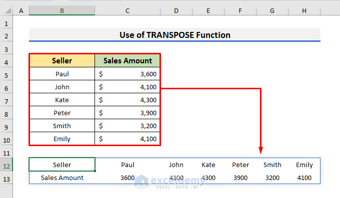
- Select B12 and enter the formula below:
=TRANSPOSE(B4:C10)
- Press Ctrl + Shift + Enter to see the result.
Read More: How to Transpose Multiple Columns to Rows in Excel
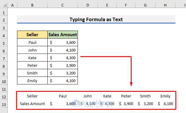
Method 3 – Enter the Formula as Text
STEPS:
- Select B12 and enter EdB4.
- Enter EdC4 in B13.
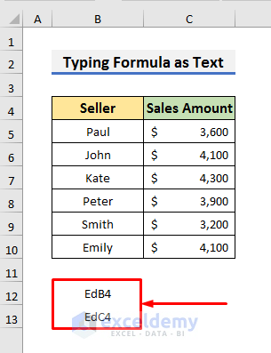
You want to see the seller in B12 and the sales amount in B13. As B4 contains seller, EdB4 was entered in B12. To see the sales amount in B13, EdC4 was used.
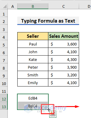
- Select B12 and B13.
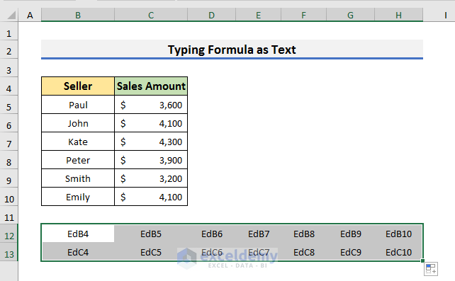
- Drag the Fill Handle to the right till column H.
- Select B12:H13.
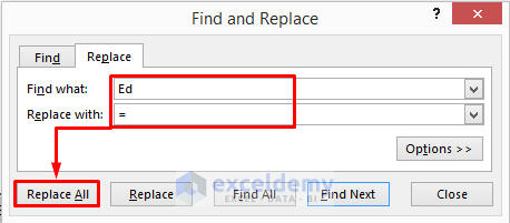
- Press Ctrl + H to open the Find and Replace box.
- Enter Ed in “Find what” and = in “Replace with”.
- Click Replace All option.
- In the message box, click OK.
This is the output.
Read More: How to Convert Multiple Rows to Columns in Excel
Method 4 – Swap a Vertical Column to a Horizontal row Using the INDEX Function in Excel
STEPS:
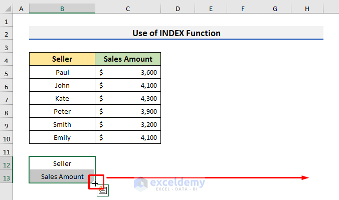
- Select B12 and enter the formula below:
=INDEX($B$4:$C$10,COLUMN(A1),ROW(A1))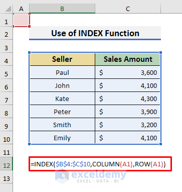
The first argument is B4:C10 (to convert to horizontal rows). COLUMN(A1) returns the column number of A1: 1. ROW(A1) returns the row number of A1: 1. The formula becomes INDEX($B$4:$C$10,1,1). B12 will store the first value in B4:C10: Seller.
- Press Enter and drag the Fill Handle down to B13.
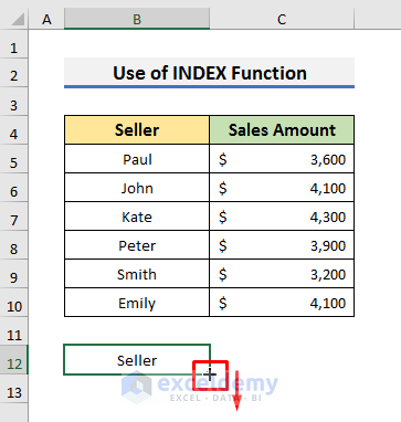
- Select B12 and B13.
- Drag the Fill Handle to the right.
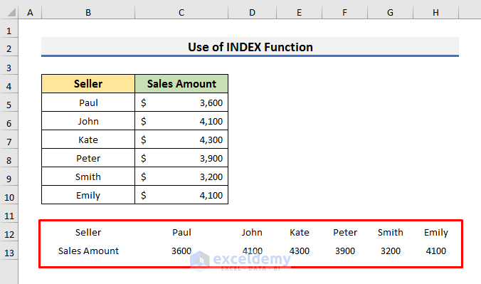
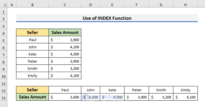
This is the output.
- This is the dataset after formatting:
Read More: How to Flip Data from Horizontal to Vertical in Excel
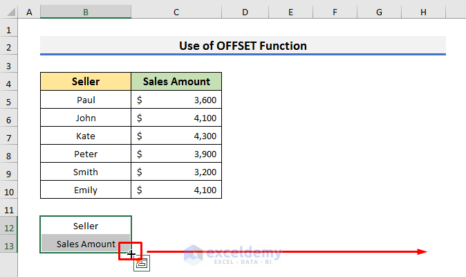
Method 5 – Applying the OFFSET Function
STEPS:
- Select B12 and enter the formula below:
=OFFSET($B$4,COLUMN(A1)-1,ROW(A1)-1)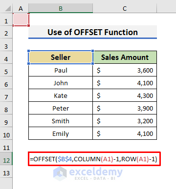
In the OFFSET function B4 is the reference. COLUMN(A1)-1 and ROW(A1)-1 denote the row and column numbers from the reference.
- Press Enter and drag the Fill Handle down.

- Select B12 and B13.
- Drag the Fill Handle to the right till Column H.
This is the output.
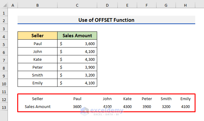
This is the dataset after formatting:

Read More: How to Move Data from Row to Column in Excel
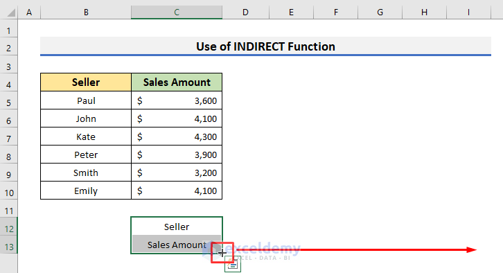
Method 6 – Transpose a Vertical Column to a Horizontal row Using the INDIRECT Function
STEPS:
- Use the formula below in C12:
=INDIRECT("B"&COLUMN()+1)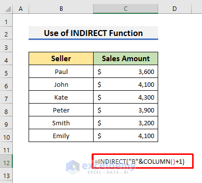
The output of COLUMN() is 3. The formula becomes INDIRECT(B4). It returns Seller in C12.
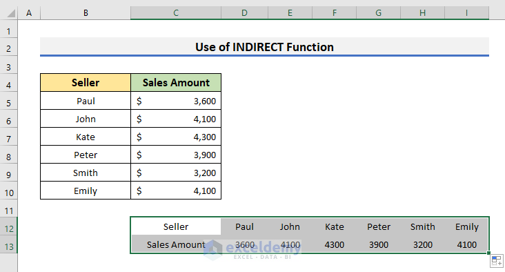
- Press Enter and use the formula below:
=INDIRECT("C"&COLUMN()+1)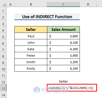
- Drag the Fill Handle to the right till Column I.
This is the output.
Read More: How to Paste Link and Transpose in Excel
Download Practice Workbook
Download the workbook.
Related Article
<< Go Back to Transpose Data in Excel | Learn Excel
Get FREE Advanced Excel Exercises with Solutions!
