How to Flip Data from Horizontal to Vertical in Excel (6 Methods)

Dataset Overview

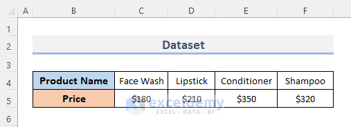
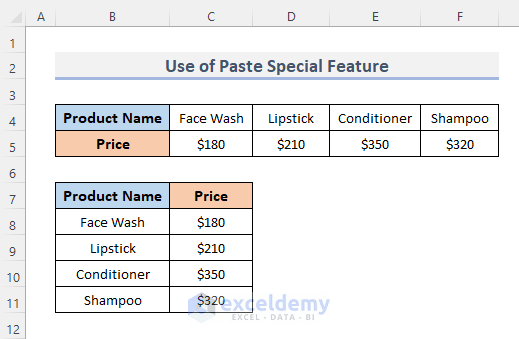
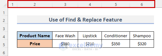
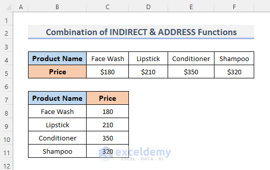
We will be working with the following dataset, which includes product names and their corresponding total prices. Our task is to rearrange the columns by flipping them and then organize them from a horizontal layout to a vertical one.

Method 1 – Using Paste Special Feature

In this first method, we will use the Excel Paste Special feature to flip data. Our main goal is to transpose the data using this feature. Transposing generates a new data arrangement where the original rows and columns are reversed. It automatically generates new variable names and provides a list of the new value labels. Excel includes a transpose feature that allows us to flip horizontal data to a vertical format.

STEPS:

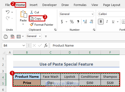
• Select the entire data that is currently arranged horizontally.
• Navigate to the Home tab in the ribbon.
• Click on Copy under the Clipboard.
  • Alternatively, you can use the keyboard shortcut Ctrl + C to copy the entire data.

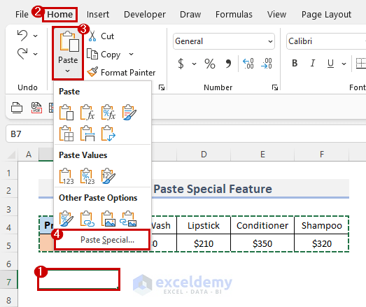
• Select the cell where you want to flip the data from horizontal to vertical. In this case, we’ll choose cell B7.
• Go back to the Home
• Click on the Paste drop-down menu under the Clipboard
• Select Paste Special.
• Alternatively, you can use the keyboard shortcut Ctrl + Alt + V to open the Paste Special

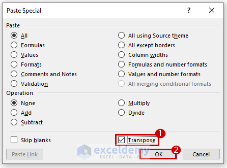
• This will display the Paste Special dialog box.
• Select the Transpose option as shown in the screenshot below.
• Click the OK button to complete the process.

• After following the instructions above, you’ll notice that the data has been flipped from horizontal to vertical.

Read More: How to Change Vertical Column to Horizontal in Excel

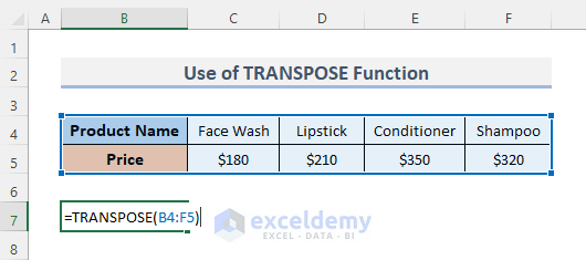
Method 2 – Using Excel TRANSPOSE Function

With the TRANSPOSE function, you can change the orientation of a group of cells from vertical to horizontal or vice versa. The TRANSPOSE function flips the direction of a specified range. Let’s follow the steps to use this function and flip the data:

STEPS:

• Select the cell where you want to flip the data. In this case, we’ll select cell B7.
• Enter the following formula into the selected cell:
  
  =TRANSPOSE(B4:F5)
  
• Press Enter.

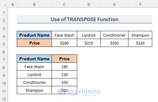
• After following these instructions, the data will be flipped from horizontal to vertical.

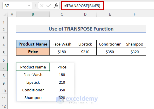
To maintain the existing format, we need to manually organize it.

Read More: How to Flip Columns and Rows in Excel

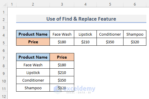
Method 3 – Applying the Find & Replace Feature 

The Excel Find & Replace feature provides a variety of sophisticated options to help you refine your search and locate specific content. While it’s possible to use this feature to flip data, it can be a bit tricky to do so.

To achieve this, follow these steps:

• Open your Excel workbook.
• Go to the File tab in the ribbon.

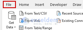
• Go backstage to the Excel menu bar.
• Click on Options.

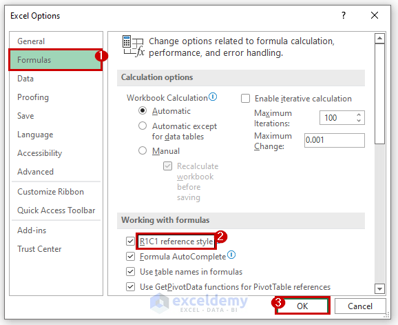
• Navigate to the Formulas section.
• Checkmark the R2C1 reference style box under the Working with formulas options.
• Click OK.

As a result, all the columns will change to numbers.

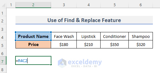
• Enter the formula into a selected cell:
  
  =R4C2
  
• This will represent the 4th row and the 2nd column which is the Product Name.

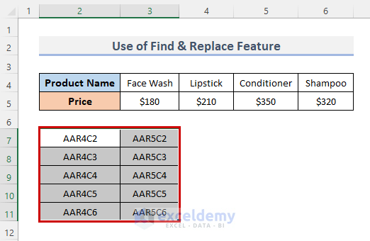
• Instead of using the equal (=) sign, we’ll reference the row and column. In our case, the reference is AA, resulting in the final output: AAR4C2.
• Drag the mouse cursor to fill the entire data range for flipping.

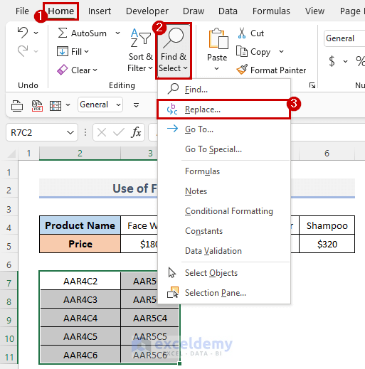
• Select the data and navigate to the Home tab.
• In the Editing group, click on the Find & Replace drop-down menu and choose Replace.
• Alternatively, you can use the keyboard shortcut Ctrl + H to open the Find & Replace dialog.

• The Find & Replace dialog box will appear.
• Enter AA in the Find what field and = in the Replace with field.
• Click Replace All.
• Click Close.

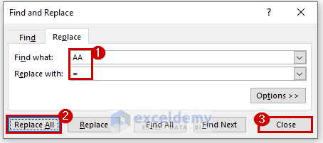
As a result, you’ve generated your flipped data.

Read More: How to Convert Multiple Rows to Columns in Excel

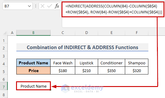
Method 4 – Combine INDIRECT and ADDRESS Functions 

STEPS:

• Choose the cell where you want to flip the data from horizontal to vertical.
• In that selected cell, enter the following formula:
  
  =INDIRECT(ADDRESS(COLUMN(B4)-COLUMN($B$4)+ROW($B$4), ROW(B4)-ROW($B$4)+COLUMN($B$4)))
  
• Press the Enter key to complete the operation.

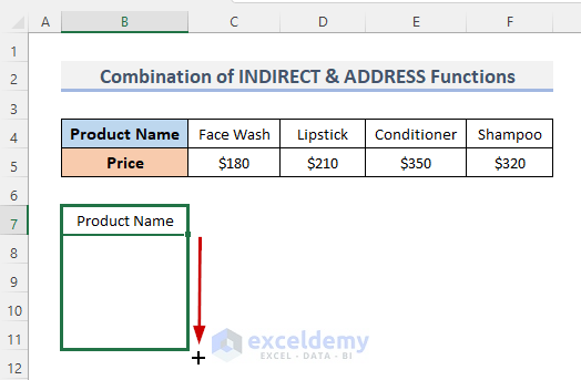
• Drag the Fill Handle down to duplicate the formula over the desired range.
• Alternatively, double-click on the plus (+) symbol to AutoFill the range.

• To replicate the formula across the range horizontally, drag the Fill Handle

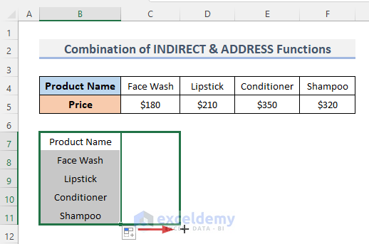
• You’ll notice that the data is now flipped from horizontal to vertical.
• Remember to manually adjust the format to maintain consistency.

Read More: How to Move Data from Row to Column in Excel

Method 5 – Applying Excel VBA Macro

STEPS:

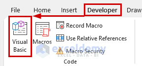
• Go to the Developer tab in the Excel ribbon.
• From the Code category, click on Visual Basic to open the Visual Basic Editor.
• Alternatively, press Alt + F11 to directly open the Visual Basic Editor.

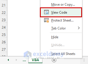
• You can also right-click on your worksheet and choose View Code to access the Visual Basic Editor.

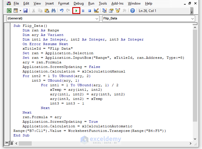
• In the Visual Basic Editor, enter the following VBA code:

VBA Code:

Sub Flip_Data()
    Dim ran As Range
    Dim ary As Variant
    Dim int1 As Integer, int2 As Integer, int3 As Integer
    On Error Resume Next
    xTitleId = "Flip Data"
    Set ran = Application.Selection
    Set ran = Application.InputBox("Range", xTitleId, ran.Address, Type:=8)
    ary = ran.Formula
    Application.ScreenUpdating = False
    Application.Calculation = xlCalculationManual
    For int2 = 1 To UBound(ary, 2)
        int3 = UBound(ary, 1)
            For int1 = 1 To UBound(ary, 1) / 2
                xTemp = ary(int1, int2)
                ary(int1, int2) = ary(int3, int2)
                ary(int3, int2) = xTemp
                int3 = int3 - 1
            Next
    Next
    ran.Formula = ary
    Application.ScreenUpdating = True
    Application.Calculation = xlCalculationAutomatic
Range("B7:C11").Value = WorksheetFunction.Transpose(Range("B4:F5"))
End Sub

• This code flips the data from horizontal to vertical.

• Click the Run Sub button or press the keyboard shortcut F5 to execute the code.

• A window will appear, asking you to specify the range of data you want to flip.

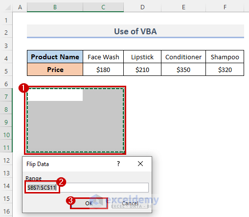
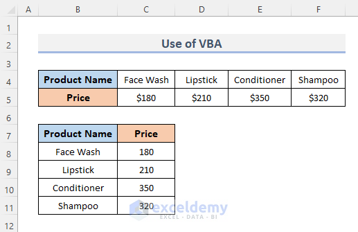
As a result, your data will be flipped from horizontal to vertical.

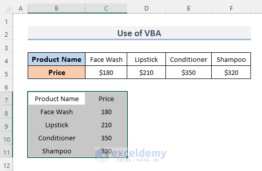
Remember to manually adjust the format to maintain consistency.

Sub Flip_Data()
    Dim ran As Range
    Dim ary As Variant
    Dim int1 As Integer, int2 As Integer, int3 As Integer

xTitleId = "Flip Data"
Set ran = Application.Selection
Set ran = Application.InputBox("Range", xTitleId, ran.Address, Type:=8)
ary = ran.Formula
Application.ScreenUpdating = False
Application.Calculation = xlCalculationManual

For int2 = 1 To UBound(ary, 2)
    int3 = UBound(ary, 1)
        For int1 = 1 To UBound(ary, 1) / 2
            xTemp = ary(int1, int2)
            ary(int1, int2) = ary(int3, int2)
            ary(int3, int2) = xTemp
            int3 = int3 - 1
      Next
Next
ran.Formula = ary
Application.ScreenUpdating = True
Application.Calculation = xlCalculationAutomatic

Range("B7:C11").Value = WorksheetFunction.Transpose(Range("B4:F5"))

Read More: Excel Macro: Convert Multiple Rows to Columns

Method 6 – Using the Power Query Tool

Power Query is an efficient tool for quickly transforming data in Excel. In this tutorial, we’ll show you how to use Power Query to convert horizontal data into vertical format.

STEPS:

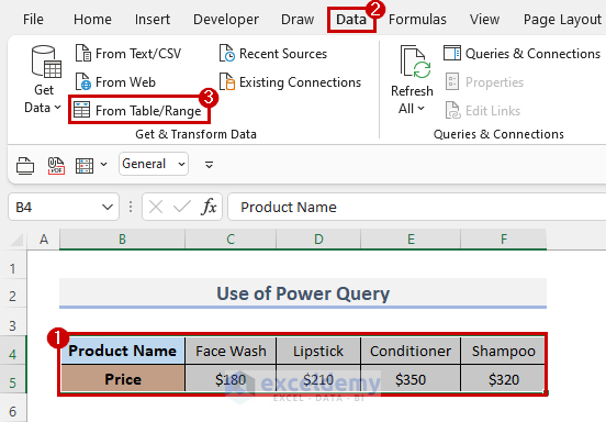
• Select the data which you want to flip.
• Go to the Data tab from the ribbon.
• Click on From Table/Range under the Get & Transform Data.

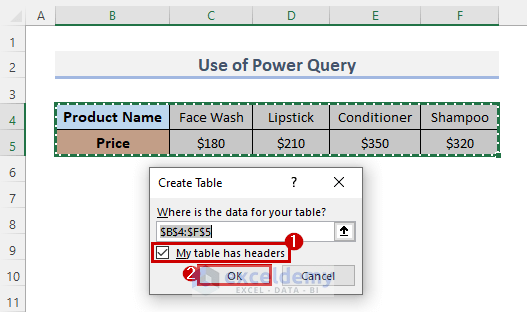
• The Create Table dialog box will appear.
• The range you selected earlier will be displayed in the Where is the data for your table? field.
• Make sure the checkbox next to My table has headers is selected.
• Click OK to proceed.

• This will open the Power Query Editor window.
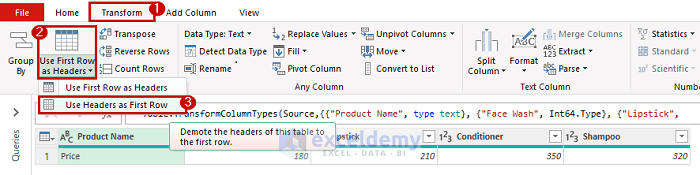
• Go to the Transform tab from the menu bar.
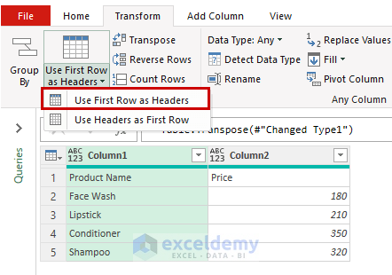
• Click on the Use First Row as Headers drop-down menu.
• Select Use Headers as First Row.
• This action will create a header for each column.

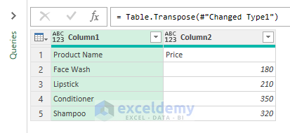
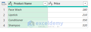
• Click on the Transpose option.

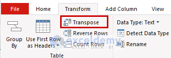
• This will flip the data from horizontal to vertical.

• Click on the Use First Row as Headers drop-down menu.
• Select Use First Row as Headers to remove the extra header.

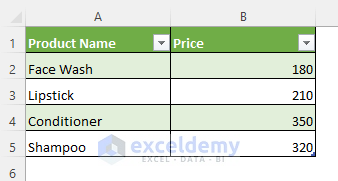
• Go to the File menu and select Close & Load.

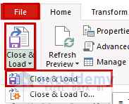
• The Power Query Editor dialog box will close, and a new sheet containing the flipped data will be loaded into the workbook.

Read More: How to Transpose Multiple Columns to Rows in Excel

Things to Keep in Mind

• Transpose Shortcut:
  • When using the Transpose feature, press Ctrl + Shift + Enter instead of just Enter.
• Select a Range:
  • Remember to choose a range of cells when transposing your dataset. The Transpose function works with larger amounts of data, not just a single data point.
• Excel VBA Code:
  • If you’re using Excel VBA code on your worksheet, make sure to save the file as an Excel Macro-Enabled Workbook(with the extension .xlsm).

Download Practice Workbook

You can download the practice workbook from here:

Related Articles

• How to Paste Link and Transpose in Excel
• Excel VBA to Transpose Array
• VBA to Transpose Multiple Columns into Rows in Excel

<< Go Back to Transpose Data in Excel | Learn Excel