Transpose Data in Excel (Applying Functions, Commands, and VBA)

Download Practice Workbook

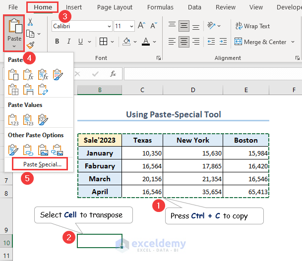
Method 1 – Using Excel Paste Special Tool to Transpose Data

Press Ctrl + C to copy the B4:E8 range.
Select B10 to transpose >> go to the Home tab >> Expand the Paste command >> select Paste Special.

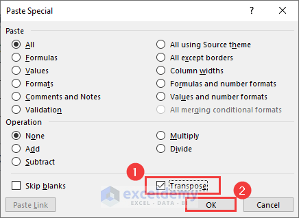
In the Paste Special dialog box, select the transpose option >> click OK.

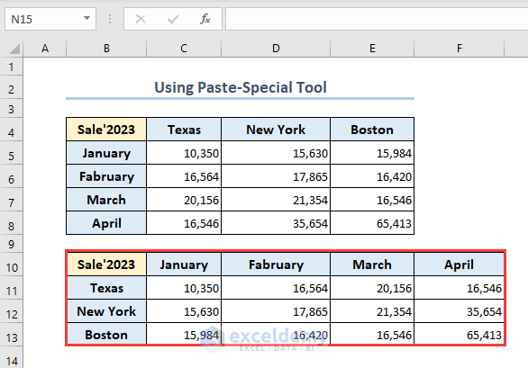
It will transpose the data from B4:E8 range to B10:F13 range.

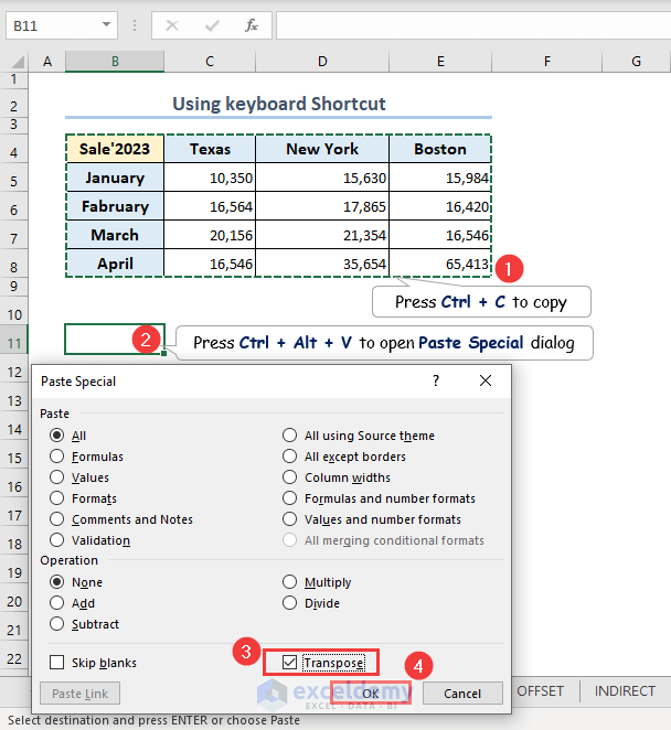
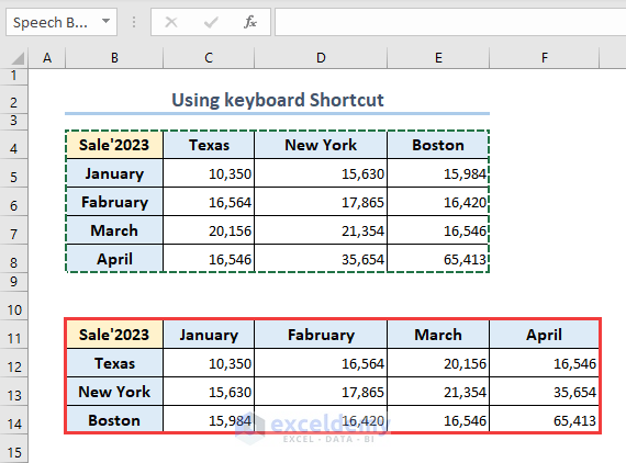
Method 2 – Applying Keyboard Shortcut for Transposing Data

The keyboard shortcut is Ctrl+ Alt + V buttons to open the Paste Special dialog box and transpose the data accordingly.

Copy the range B4:E8.
Select B11 cell (transpose location) >> press Ctrl+ Alt + V to open the Paste Special dialog.
Select Transpose from the Paste Special dialog>> click OK.

You’ll get the transposed result in the B11:F14 range.

Method 3 – Inserting TRANSPOSE Function Switch Rows to Columns

You can use the dedicated function named the TRANSPOSE function to transpose a range/table. It uses an array as an argument and returns a range.

Enter the following formula in B10 to obtain the transposed result.

=TRANSPOSE(B4:E8)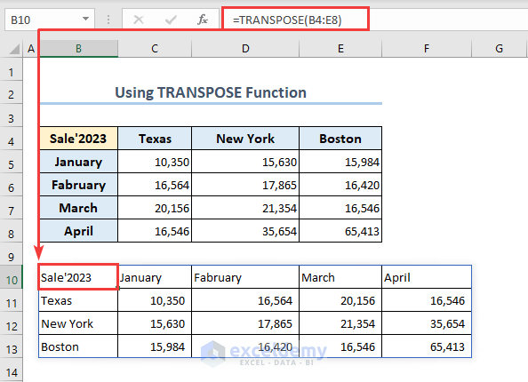

Method 4 – Applying Excel OFFSET Function to Transpose Data

The OFFSET function is applicable to transpose data, it works based on reference argument. To apply the OFFSET function, we must set the rows and column numbers to transpose a dataset.

Enter B10=0, C10=1, D10=2, E10=3 and F10=4 as the number of rows.
Enter A11=0, A12=1, A13=2 and A14=3 as the number of columns.
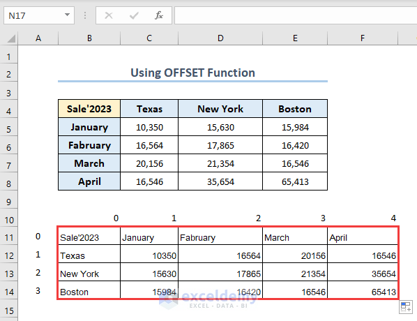
Enter the following formula in the B11 cell containing the OFFSET

=OFFSET($B$4,B$10,$A11)

Use the Fill Handle to autofill the data horizontally and vertically.

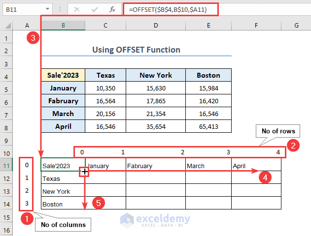
You will get the transposed data in B11:F14.

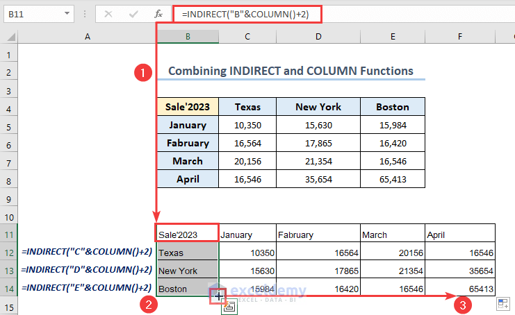
Method 5 – Combining INDIRECT and COLUMN Functions

The combination of INDIRECT and COLUMN functions can transpose a dataset. The INDIRECT function Store data from the reference specified by a text string whereas the COLUMN function shows the number of columns.

Enter the following formulas containing the INDIRECT function with the COLUMN function in the cells B11, B12, B13 and B14.

=INDIRECT("B"&COLUMN()+2)

=INDIRECT("C"&COLUMN()+2)

=INDIRECT("D"&COLUMN()+2)

=INDIRECT("E"&COLUMN()+2)

From the formula, COLUMN()= 2 that dictates (“B”&COLUMN()+2) = B4.
The INDIRECT function picks the data of the B4 Similarly call the data of C4, D4 and E4.
We will get the transposed data in the B11:F14 range after using the Fill Handle tool.

Click to get detailed view of the image

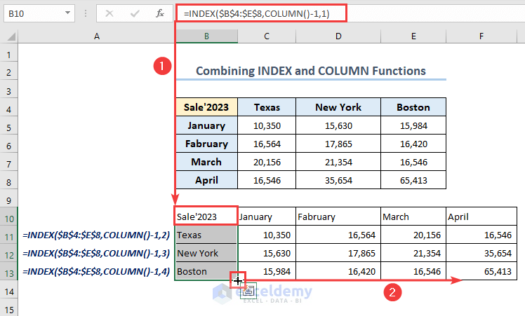
Method 6 – Merging Excel INDEX and COLUMN Functions

We can combine INDEX and COLUMN functions to transpose a dataset. The INDEX function returns a certain reference or value of the cell of a particular row and column whereas the COLUMN function picks up the column number.

Use the following formulas in the cells B10, B11, B12 and B13.

=INDEX($B$4:$E$8,COLUMN()-1,1)

=INDEX($B$4:$E$8,COLUMN()-1,2)

=INDEX($B$4:$E$8,COLUMN()-1,3)

=INDEX($B$4:$E$8,COLUMN()-1,4)

From the formula of the B10 cell, COLUMN()=2 and COLUMN()-1=2-1=1 is the row number.
We get Sale’2023 in the cell B10. We get the data in the cell B11, B12 and B13.
We will get the transposed result in the B10:F13 range after using the Fill Handle.

Click to get detailed view of the image

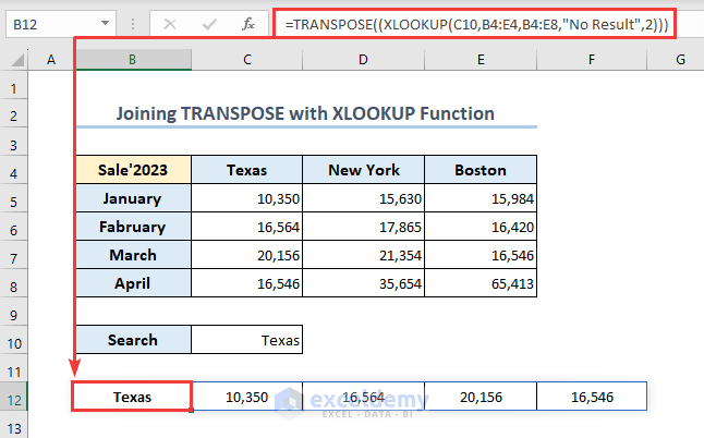
Method 7 – Joining TRANSPOSE and XLOOKUP Functions

By merging the XLOOKUP function with the TRANSPOSE function, we can transpose a specific row or column. The XLOOKUP function can be used if you are looking for a specific value.

Enter the following formula in the cell B12 to obtain the transposed results for Texas.

=TRANSPOSE((XLOOKUP(C10,B4:E4,B4:E8,"No Result",2)))

The XLOOKUP function finds the C10 = Texas in the B4:E4. It gathers the data from B4:E8. It will show No Result if it is unable to find a result. 2 is for the wildcard character match.

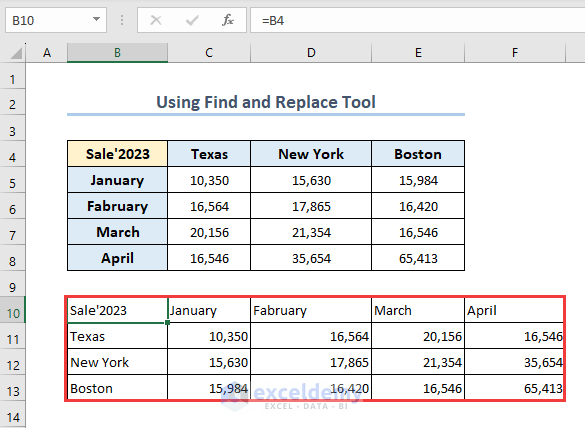
Method 8 – Using Find and Replace Feature to Shift Rows to Columns

Enter TB4, TC4, TD4 and TE4 in the B10, B11, B12 and B13 cells respectively.
Use the Fill Handle tool to autofill B10:F13.

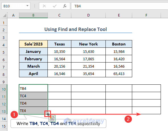
After getting the data in the B10:F13 cell, press Ctrl + H to get the Find and Replace tool.
Enter T in the Find what field and = in the Replace with field from the Replace menu.
Click on Replace All.

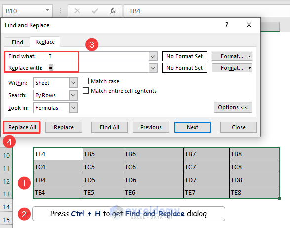
We will get the transposed result in B10:F13.

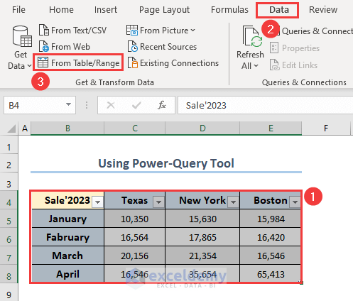
Method 9 – Using Power Query Tool to Transpose Columns to Rows

Select the dataset >> go to the Data tab >> click on From Table/Range.

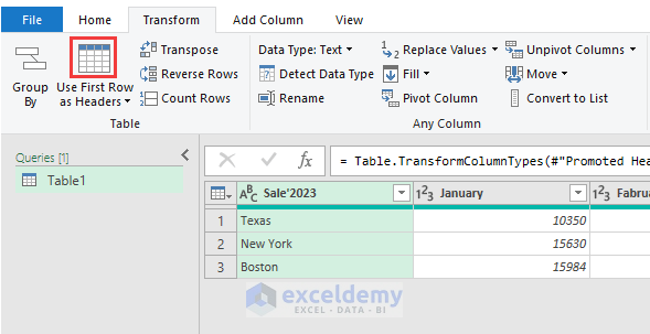
In the Power Query window, click as follows, Transform tab >> Use Headers as First Row option >> Transpose.

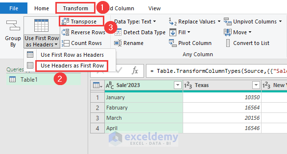
Select Use First Row as Headers.

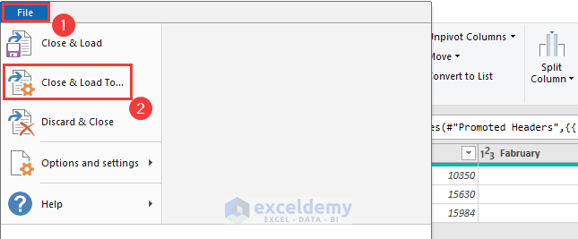
Go to the File menu >> select Close and Load To.

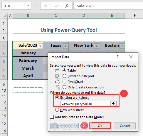
In the Import Data dialog box, select the Existing Worksheet and B10 cell in the PowerQuery worksheet >> click OK.

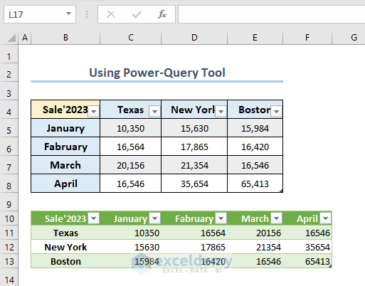
We will get the transposed data in B10:F13.

Method 10 – Applying VBA Macro Transpose Multiple Rows to Columns

VBA has a Transpose property that converts rows to columns with a simple code. You can modify the code based on your requirements.

Enter the codes in the Module and run by clicking the play icon or pressing F5.

Sub TransposeData()

    Dim Rng As Range
    Dim lastRow, firstCol As Long
    
    Set Rng = Selection
    Rng.Copy
    
    lastRow = Selection.Rows(Selection.Rows.Count).Row
    firstCol = Selection.Columns(1).Column
    
    Cells(lastRow + 2, firstCol).PasteSpecial Transpose:=True
    Application.CutCopyMode = False

End Sub

Frequently Asked Questions(FAQs)

Q. Does Excel VBA have transpose function?

No, VBA has no dedicated function named TRANSPOSE. However, there is a Transpose property under the VBA Paste Special feature that can convert rows to columns.

Q. Where is the TRANSPOSE function in Excel?

Excel also has a built-in function in the Paste Special dialog. Go to the Home tab >> Expand the Paste command >> Select the Paste Special tool >> Select Transpose from the Paste Special dialog.

Q. Can VBA update transpose values when data changes?

Yes, by adding VBA code in a worksheet module with a Change event, you can update automatically when data changes.

Transpose in Excel: Knowledge Hub

<< Go Back to Learn Excel

Get FREE Advanced Excel Exercises with Solutions!