How to Paste Link and Transpose in Excel (8 Quick Ways)

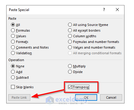
When in Paste Special, if you click on the Transpose option, the Paste Link option is automatically disabled. However, there are still ways to use them at the same time.

How to Paste Link and Transpose in Excel: 8 Ways

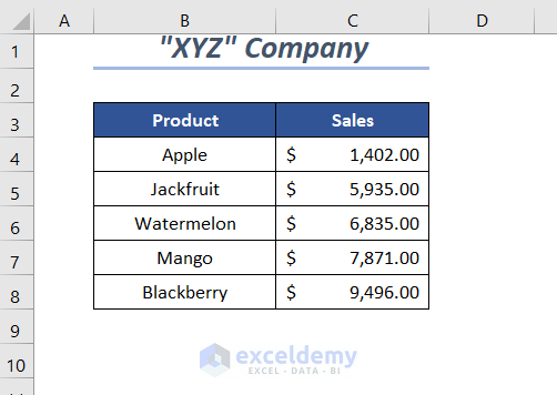
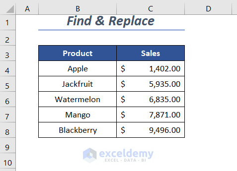
Paste Link copies the reference to the main source instead of copying only values, allowing you to track the changes between the original and the copy. Transpose allows you to paste data where rows become columns and columns become rows. We will use the following table to combine the features.

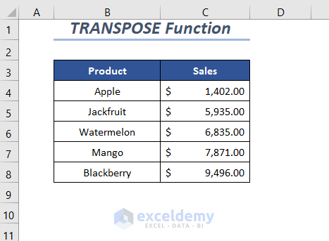
Method 1 – Using the TRANSPOSE Function to Paste Link and Transpose in Excel

We have a simple dataset that we will transpose.

Copying the Formatting:

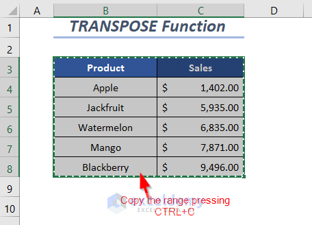
• Copy the dataset by pressing Ctrl + C.

• Select the cell where you want to paste the values and then open the Paste Special dialog box by pressing Alt, E, S one by one.

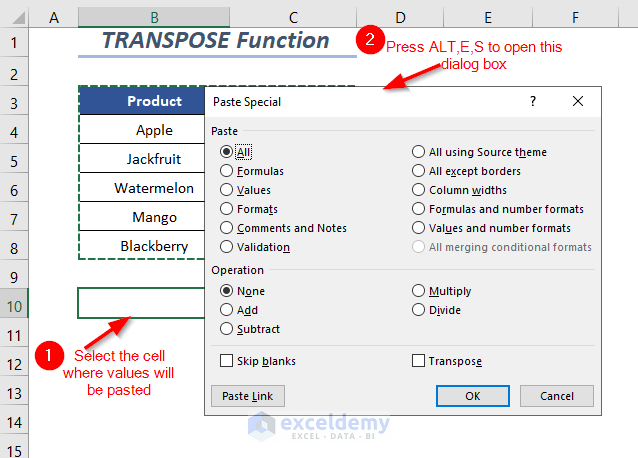
• Check the Formats option and the Transpose option and then press OK.

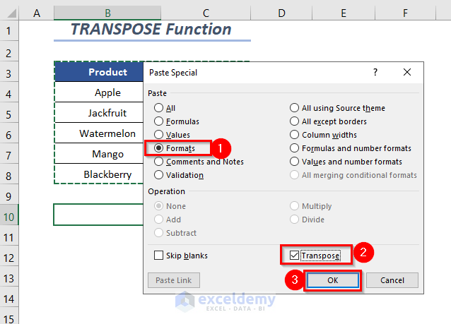
• We will get the following transposed formats of the dataset.

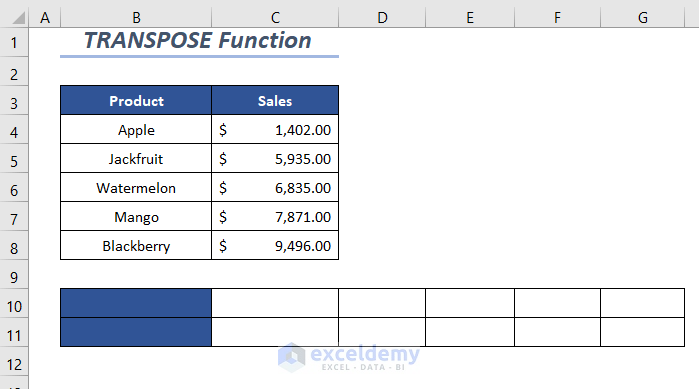
Copying the Values:

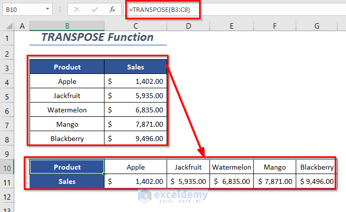
• Paste the values as links by using the following formula.

TRANSPOSE will convert the vertical range B3:C8 to the horizontal range.

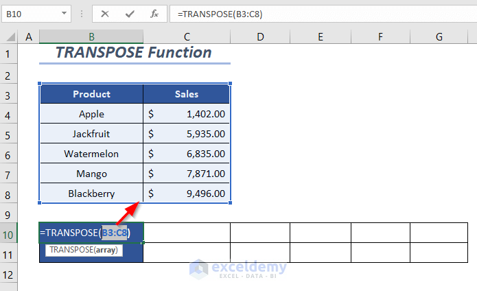
• Here’s the result.

If you use a version other than Microsoft Excel 365, you have to press Ctrl + Shift + Enter instead of Enter to apply the TRANSPOSE function.

Read More: How to Move Data from Row to Column in Excel

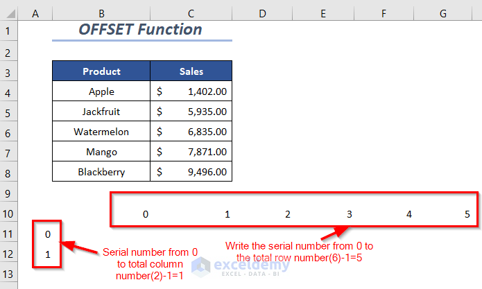
Method 2 – Using the OFFSET Function to Paste Link and Transpose

We’ll use the same dataset.

Steps

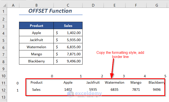
• Write the serial numbers from 0 to the total row number-1 (so until 5, as there are six rows) to the top of the area where we will paste the data and use the serial numbers from 0 to the total column number-1 (or 1, as there are two columns) to the left of the designated area.

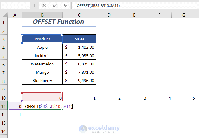
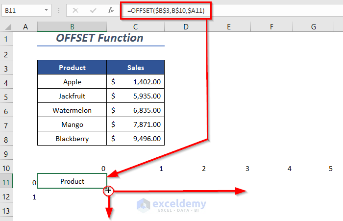
• Use the following formula in cell B11

$B$3 is the cell reference from which it starts moving, B$10 (using the $ symbol before Row 10 fixes this row) is the number of rows it moves downwards and $A11 (using the $ symbol before Column A fixes this column) is the number of columns it moves to the right. B$10 and $A11 both are zero, so the function provides the value in the cell $B$3.

• Press Enter, then drag down and to the right the Fill Handle tool.

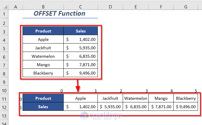
• Copy the formatting style to those pasted values by following Method 1.

• Here’s the result.

Read More: How to Flip Data from Horizontal to Vertical in Excel

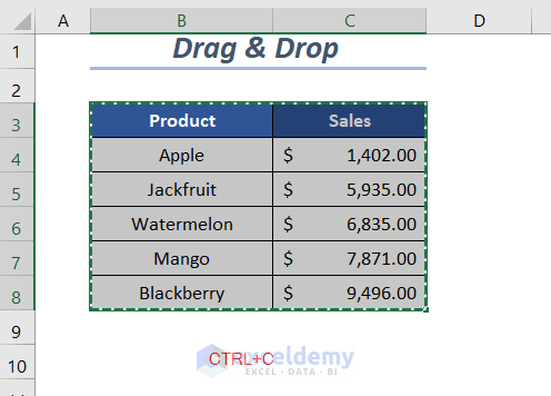
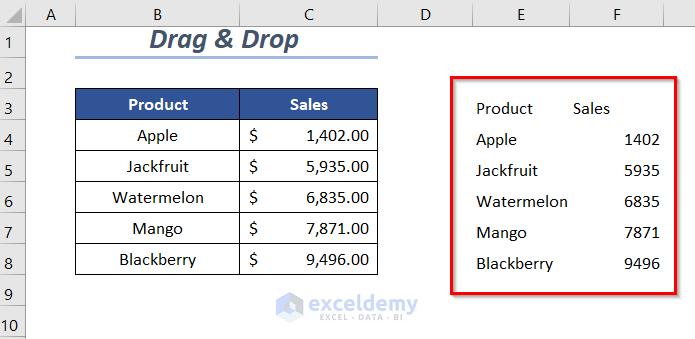
Method 3 – Paste Link and Transpose in Excel by Dragging and Dropping

We’ll use the same dataset as before.

Steps:

• Copy the dataset by pressing Ctrl + C.

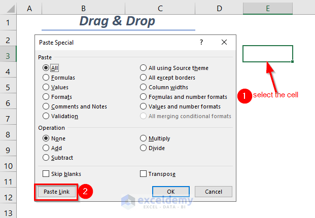
• Select the cell where you want to paste the values.
• Click on the Paste Link option of the Paste Special dialog box.

• We have pasted the data source as links.

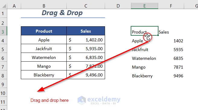
• Drag each of the cells from here and drop them to create a transposed dataset.
• Select the first cell value of cell E3 and drag it to cell B10.
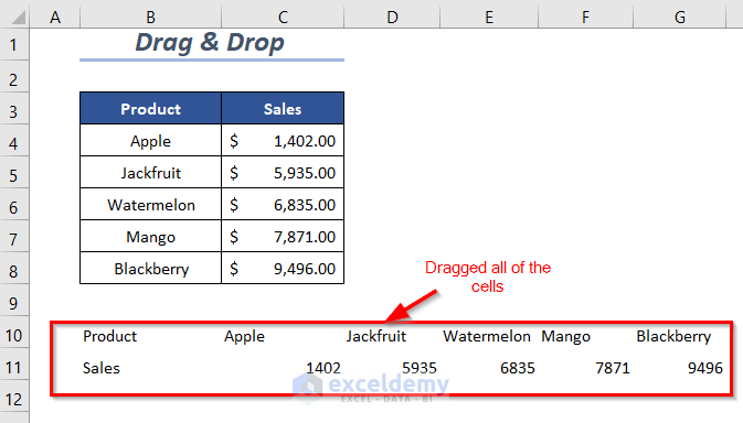
• Repeat for other cells with their respective row and column numbers.

• After dragging each cell of Column E to Row 10 and Column F to Row 11, we get the following linked values.

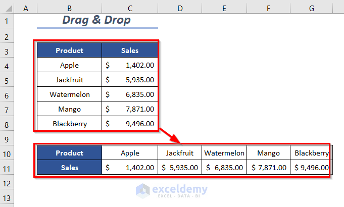
• Copy and transpose the formatting style from the table following Method 1.

Read More: How to Change Vertical Column to Horizontal in Excel

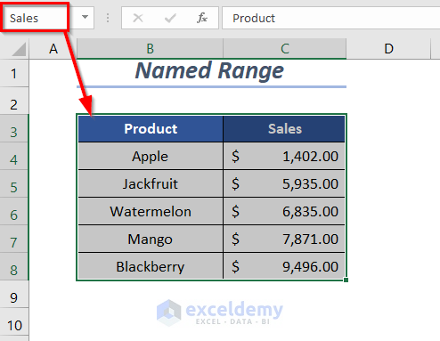
Method 4 – Using a Named Range to Paste Link and Transpose

We have named the range as Sales.

Steps:

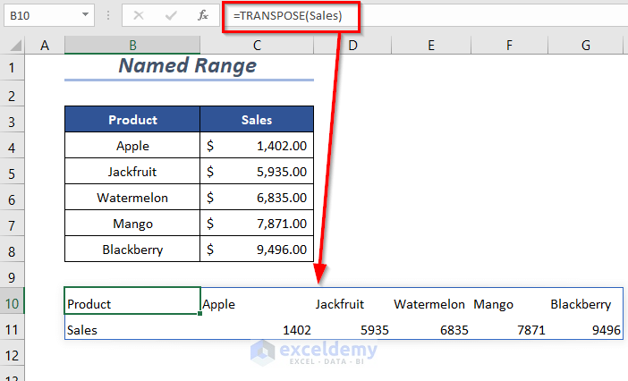
• Use the following formula in cell B10

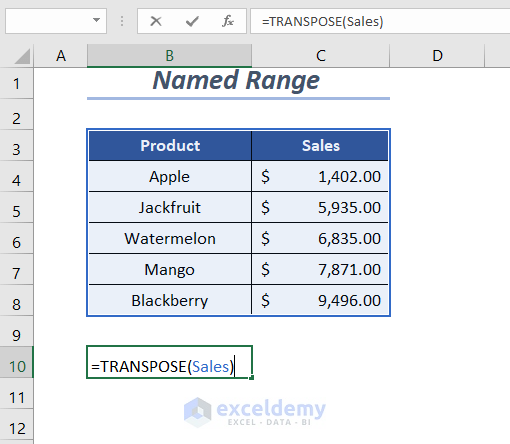
• Hit Enter.

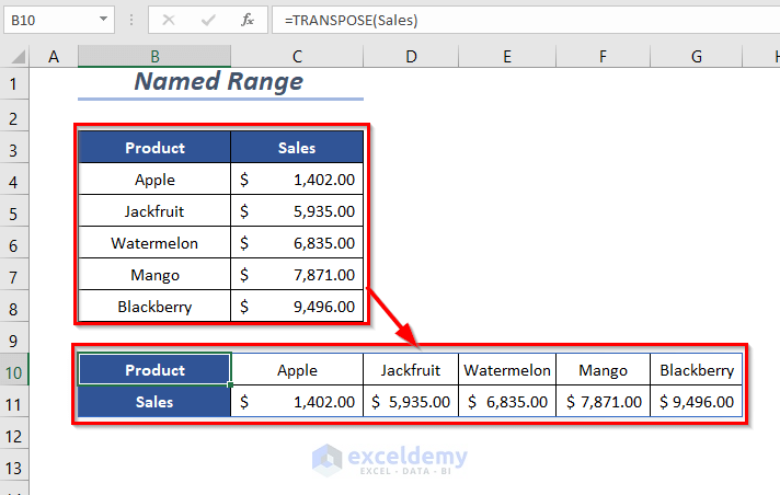
• Follow Method 1 to have the formatting styles in the transposed dataset.

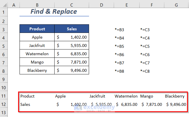
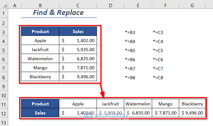
Method 5 – Using the Find & Replace Option to Paste Link and Transpose

We’ll use the same basic dataset.

Steps:

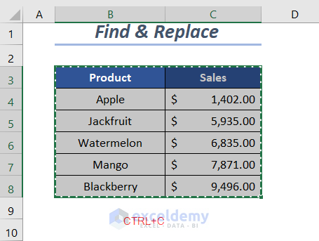
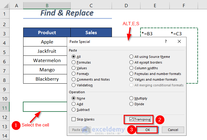
• Copy the dataset by pressing Ctrl + C.

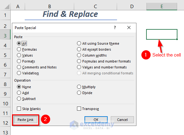
• Select the cell where you want to paste the values.
• Click on the Paste Link option of the Paste Special dialog box.

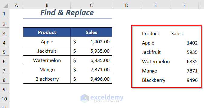
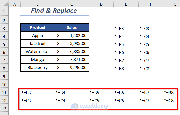
• We have pasted the data source as links.

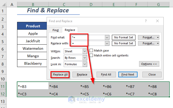
• Select the pasted dataset and hit Ctrl + H to go to Find & Select > Replace.

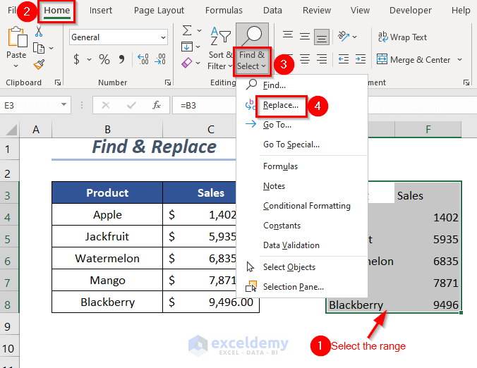
• Then the Find and Replace dialog box will open up.
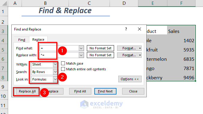
• Use the following settings:

Find what → =
Replace what → *=
Within → Sheet
Search → By Rows
Look in → Formulas

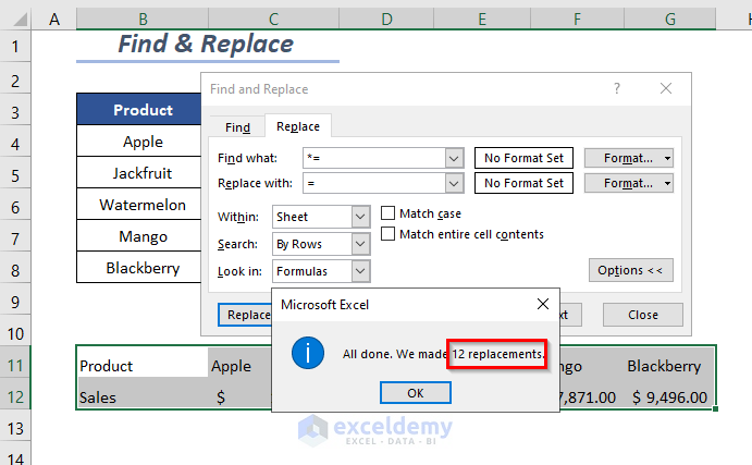
• Select the Replace All option.

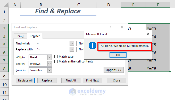
• You will get a message box notifying you about the total number of replacements.

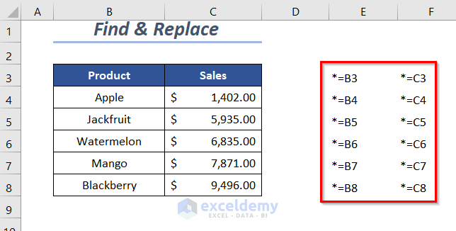
• We have converted the formulas in the cells to text strings by replacing = with *= and now we will transpose it.

• Copy the new dataset by pressing Ctrl + C.

• Select the cell where you want to paste the values, click on the Transpose option of the Paste Special dialog box and hit OK.

• We’ll get the transposed strings. Select them.

• Open the Find and Replace dialog box again, put *= in the Find what box and = in the Find what box, and hit Replace All.

• You’ll get a message box, so click OK.

• Here’s the result.

• Copy the cell formatting and transpose it from the original dataset (as in Method 1).

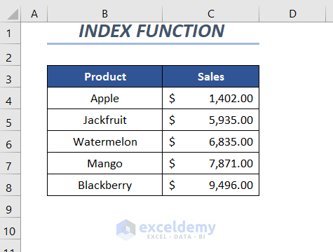
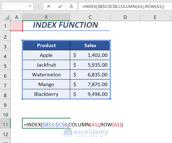
Method 6 – Using the INDEX Function to Paste Link and Transpose in Excel

We’ll start with the same dataset as before.

Steps:

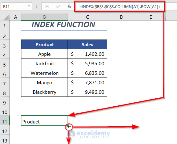
• Use the following formula in cell B11:

• Press Enter.
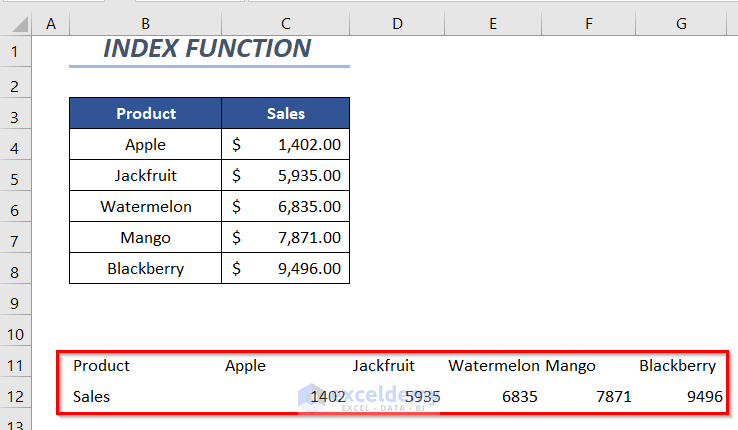
• Drag the Fill Handle down and to the right.

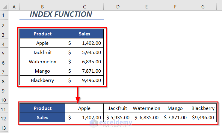
• Here’s the result.

• Follow the first part of Method 1 to transpose the cell formatting from the original.

Read More: How to Transpose Multiple Columns to Rows in Excel

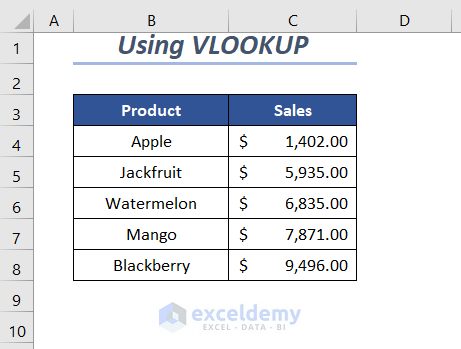
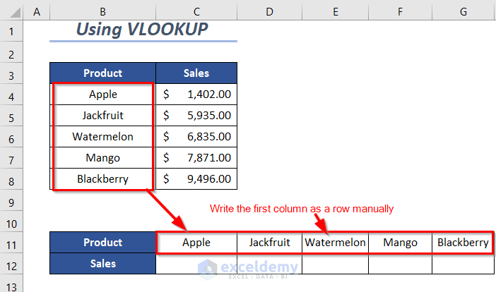
Method 7 – Using the VLOOKUP Function to Paste Link and Transpose

We’re starting with a basic dataset.

Steps:

• We have copied the formatting style following Method 1.
• Manually transpose the first column by entering or copying values.

• Use the following formula in cell C12:

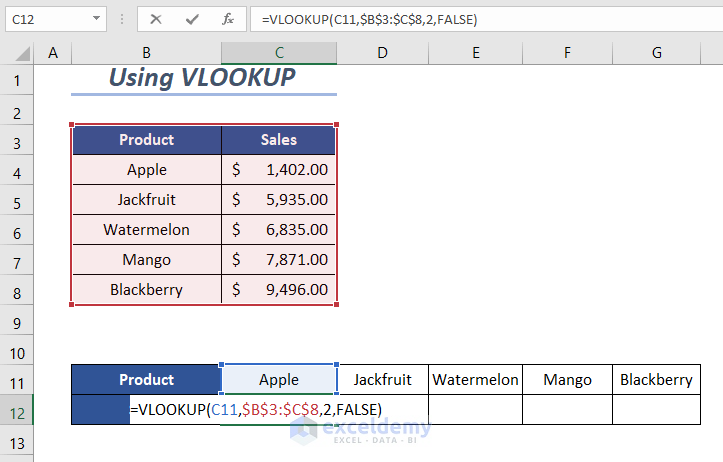
• Press ENTER and drag the Fill Handle to the right.

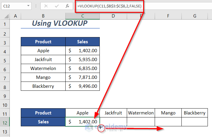
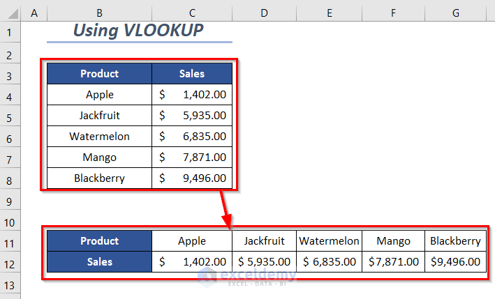
• Here’s the result.

Method 8 – Using the INDEX and MATCH Functions to Paste Link and Transpose in Excel

• We have copied the formatting style and manually transposed the first column.

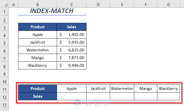
• Use the following formula in cell C12:

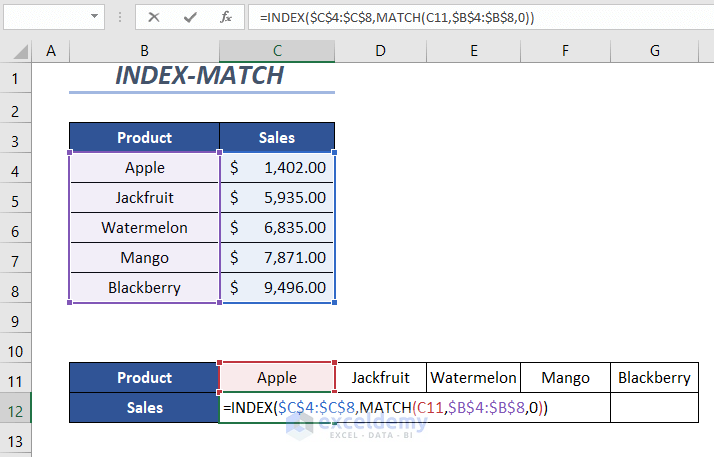
• Press Enter and drag the Fill Handle tool to the right.

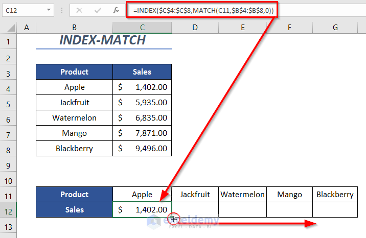
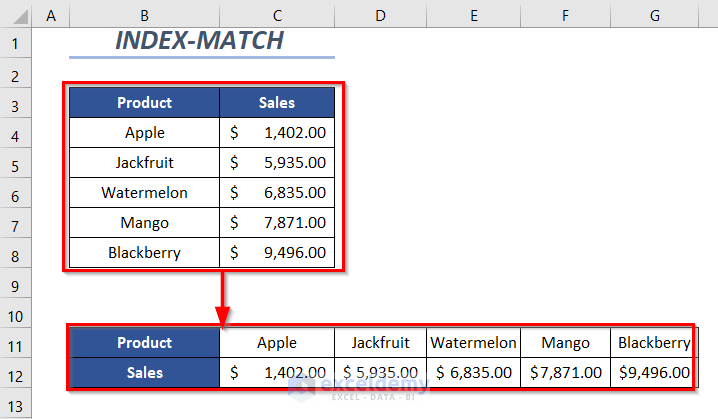
• You will get the transposed and linked dataset.

If you use a version other than Microsoft Excel 365, you have to press Ctrl + Shift + Enter instead of Enter to apply the formula.

Read More: How to Convert Multiple Rows to Columns in Excel

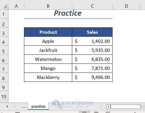
Practice Section

We have provided a Practice section like below in a sheet named Practice.

Download the Practice Workbook

Related Articles

• Excel VBA to Transpose Array
• VBA to Transpose Multiple Columns into Rows in Excel

<< Go Back to Transpose Data in Excel | Learn Excel