If you are looking for some of the easiest ways to convert multiple rows to columns in Excel, then you will find this article helpful.
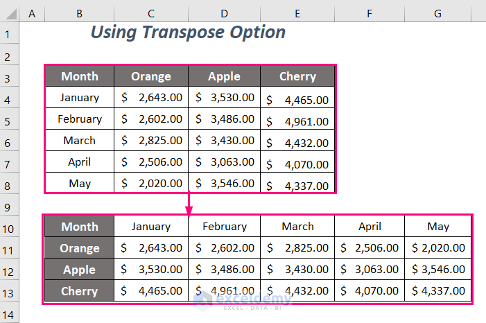
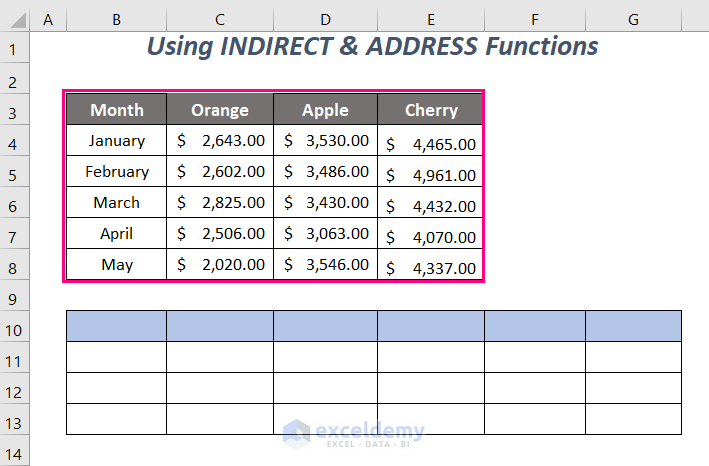
In the sample dataset that we will use to demonstrate the methods, we have some records of sales for some products for the months from January to May. Let’s convert the rows into columns so that we can visualize the months as column headers.
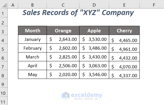
We have used Microsoft Excel 365 version here, but you can use any other versions according to your convenience.
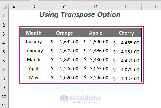
Method 1 – Using the Transpose Option
We can use the Transpose option within Paste options to convert the following multiple rows into columns easily.
Steps:
- Copy the whole range of the dataset by pressing CTRL+C.
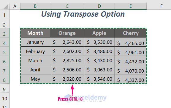
- Choose the cell where you want to have the output, Right-click on your mouse, and select the Transpose option from the Paste Options.
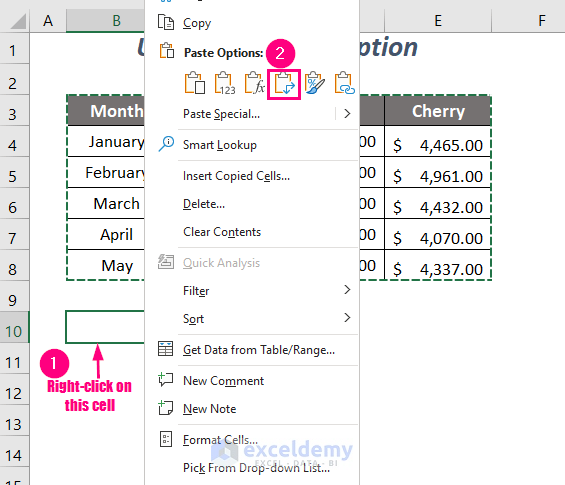
The data is transposed, which means the rows are converted into columns.
Read More: How to Transpose Multiple Columns to Rows in Excel
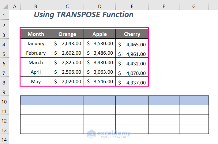
Method 2 – Using the TRANSPOSE Function
We can use an array function, the TRANSPOSE function, to convert multiple rows into multiple columns. To gather the data, we have also formatted another table below the main dataset.
Steps:
- Enter the following formula in cell B10:
=TRANSPOSE(B3:E8)Here, TRANSPOSE will change the rows of the range B3:E8 into columns simultaneously.
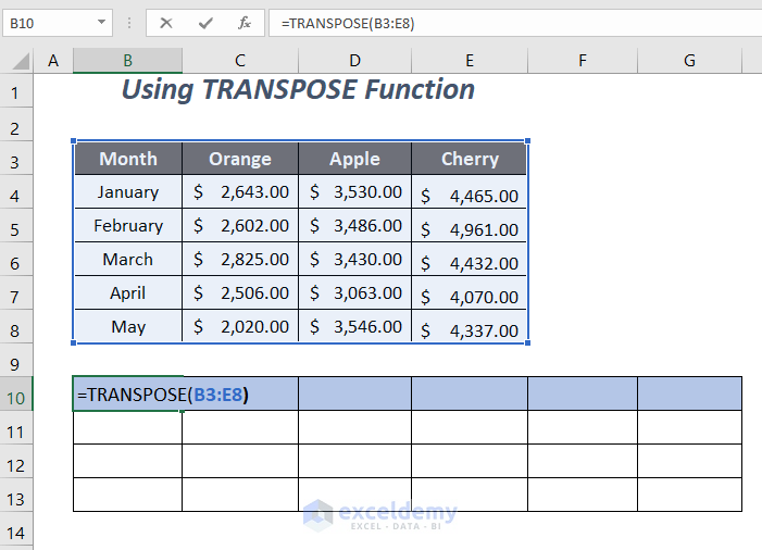
- Press ENTER. *
The conversion of the rows into columns is performed, like in the following figure.
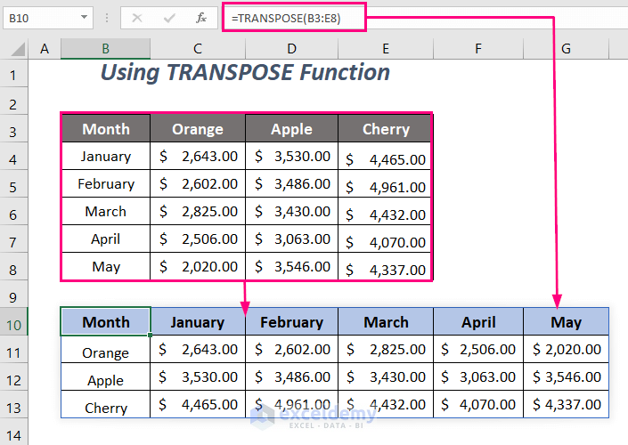
* Press CTRL+SHIFT+ENTER instead of ENTER for other versions except for Microsoft Excel 365.
Method 3 – Using INDIRECT and ADDRESS Functions
We can use the INDIRECT, ADDRESS, ROW, and COLUMN functions to transform our rows into columns.
Steps:
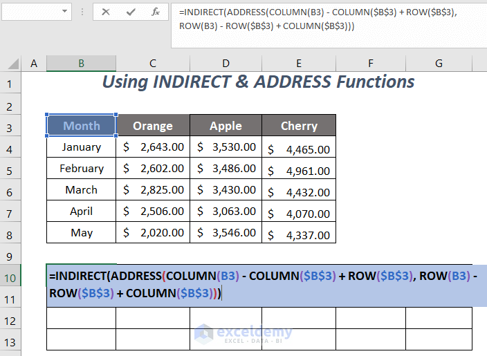
- Use the following formula in cell B10:
=INDIRECT(ADDRESS(COLUMN(B3) - COLUMN($B$3) + ROW($B$3), ROW(B3) - ROW($B$3) + COLUMN($B$3)))Here, B3 is the starting cell of the main dataset.
COLUMN(B3)→returns the column number of cellB3
Output → 2
COLUMN($B$3)→returns the column number of cell$B$3(the absolute referencing will fix this cell)
Output → 2
ROW($B$3)→returns the row number of cell$B$3(the absolute referencing will fix this cell)
Output → 3
ROW(B3) →returns the row number of cellB3
Output → 3
COLUMN(B3) - COLUMN($B$3) + ROW($B$3)becomes
2-2+3 → 3
ROW(B3) - ROW($B$3) + COLUMN($B$3)becomes
3-3+2 → 2
ADDRESS(COLUMN(B3) - COLUMN($B$3) + ROW($B$3), ROW(B3) - ROW($B$3) + COLUMN($B$3))becomes
ADDRESS(3, 2) →returns the reference at the intersection point ofRow 3andColumn 2
Output → $B$3
INDIRECT(ADDRESS(COLUMN(B3) - COLUMN($B$3) + ROW($B$3), ROW(B3) - ROW($B$3) + COLUMN($B$3)))becomes
INDIRECT(“$B$3”)→ returns the value of the cell $B$3.
Output → Month
- Press ENTER.
- Drag the Fill Handle tool to the right side and down.
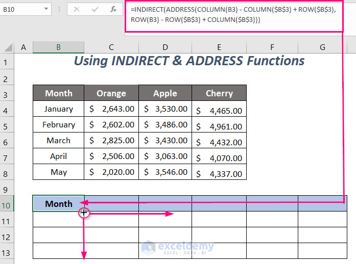
The formula will change multiple rows of the main dataset into multiple columns.

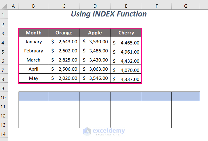
Method 4 – Using the INDEX Function
We can also use the combination of the INDEX, COLUMN, and ROW functions.
Steps:
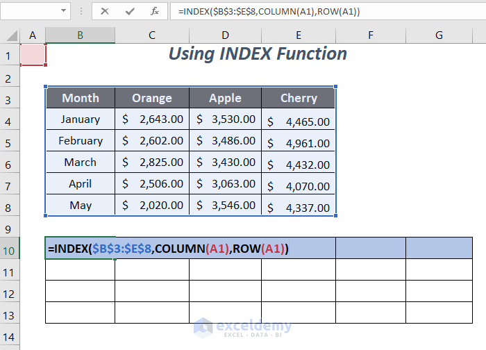
- Apply the following formula in cell B10.
=INDEX($B$3:$E$8,COLUMN(A1),ROW(A1))Here, $B$3:$E$8 is the range of the dataset, and A1 is used to get the first row and column number of this dataset. We use the column number for the row number argument and row number as the column number argument to change the rows into columns easily by feeding these values into the INDEX function.
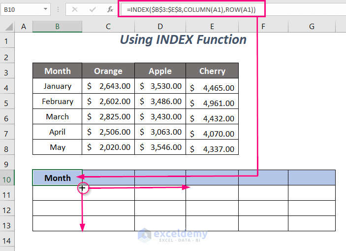
- Press ENTER.
- Drag the Fill Handle tool to the right side and down.
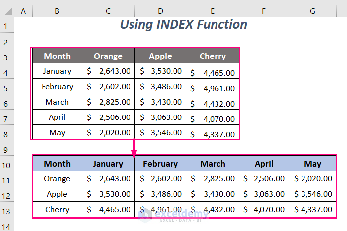
We get the conversion of the rows into columns like in the following figure.
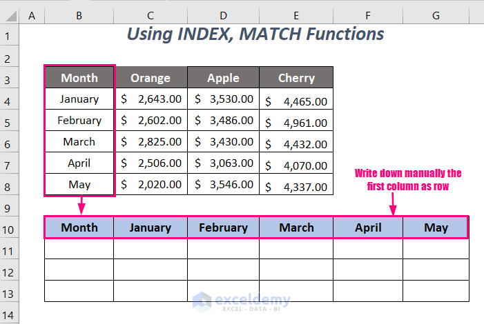
Method 5 – Using the INDEX-MATCH Formula
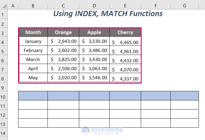
Steps:
- Transpose the first column as the first row of the new table manually.
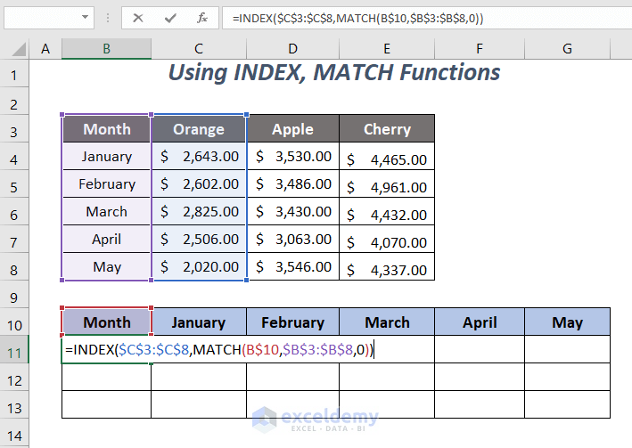
- Enter the following formula in cell B11:
=INDEX($C$3:$C$8,MATCH(B$10,$B$3:$B$8,0))Here, $C$3:$C$8 is the second column of the dataset, and $B$3:$B$8 is the first column of the dataset.
MATCH(B$10,$B$3:$B$8,0)becomes
MATCH(“Month”,$B$3:$B$8,0)→ returns the row index number of the cell with a string Month in the range $B$3:$B$8
Output → 1
INDEX($C$3:$C$8,MATCH(B$10,$B$3:$B$8,0))becomes
INDEX($C$3:$C$8,1)→ returns the first value of the range $C$3:$C$8
Output → Orange
- Press ENTER and drag the Fill Handle tool to the right side.
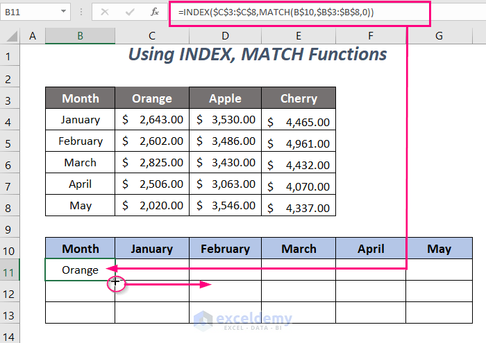
We will get the second column of the main dataset as the second row.
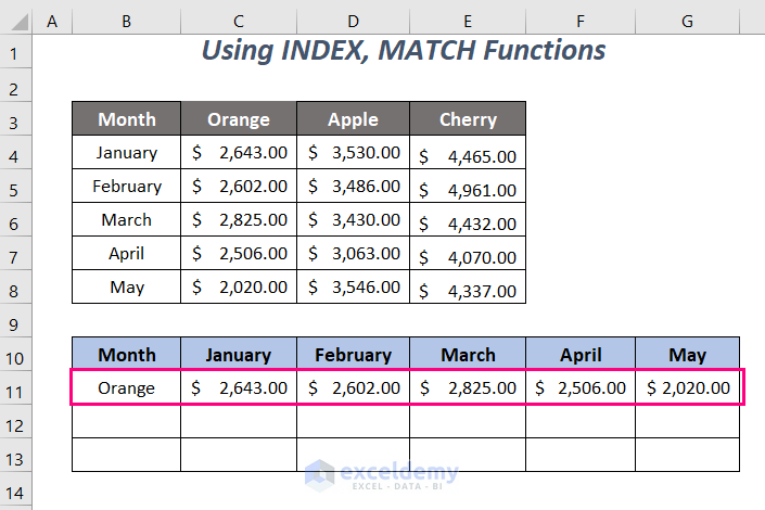
- Similarly, apply the following formulas to finish the rest of the conversion:
=INDEX($D$3:$D$8,MATCH(B$10,$B$3:$B$8,0))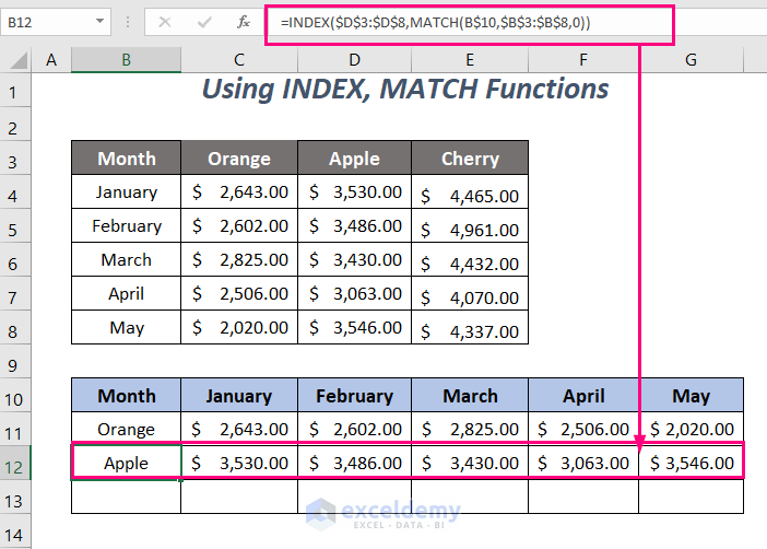
=INDEX($E$3:$E$8,MATCH(B$10,$B$3:$B$8,0))We get all of the rows of the first dataset as the columns in the second dataset.

Read More: How to Flip Data from Horizontal to Vertical in Excel
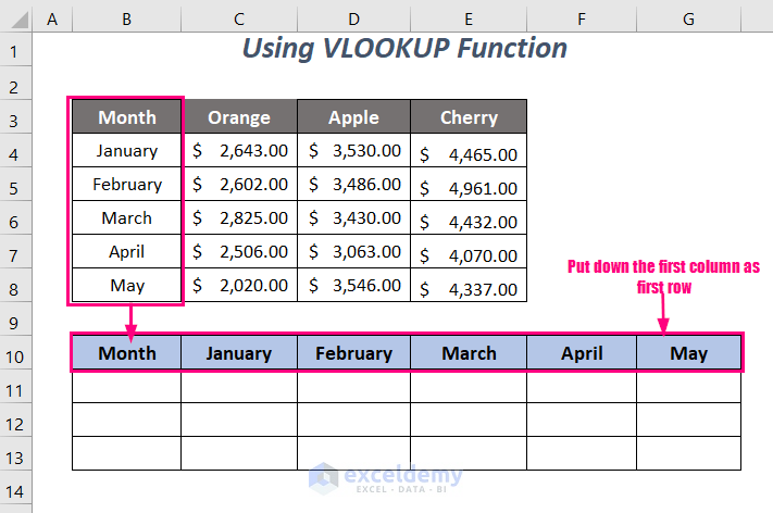
Method 6 – Using the VLOOKUP Function
Steps:
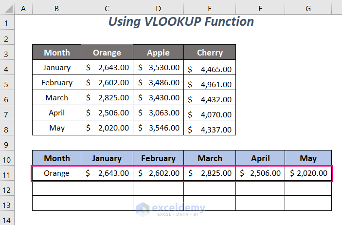
- Transpose the first column as the first row of the new dataset manually.
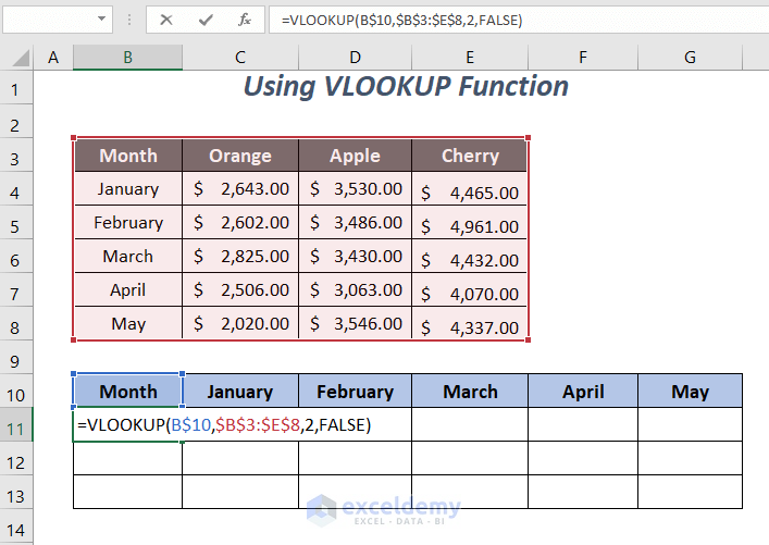
- Enter the following formula in cell B11:
=VLOOKUP(B$10,$B$3:$E$8,2,FALSE)Here, $B$3:$E$8 is the range of the dataset, B$10 is the lookup value, and 2 is for looking at the value in the second column of the dataset.
- Press ENTER and drag the Fill Handle tool to the right side.
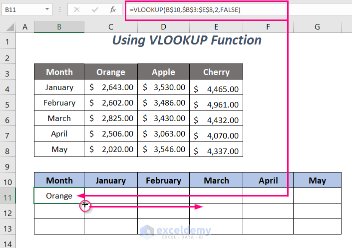
We get the second column of the main dataset as the second row.
- In the same way, use the formulas given below to complete the rest of the conversion:
=VLOOKUP(B$10,$B$3:$E$8,3, FALSE)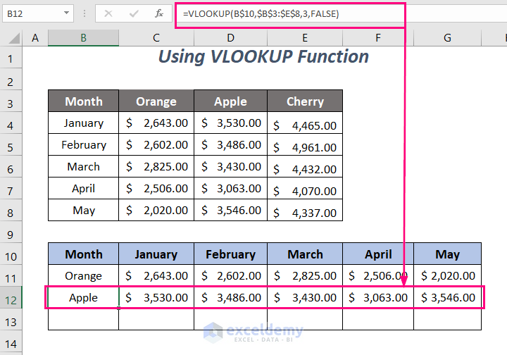
=VLOOKUP(B$10,$B$3:$E$8,4, FALSE)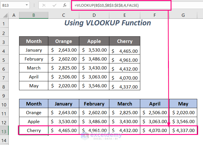
Read More: How to Move Data from Row to Column in Excel
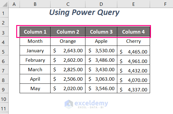
Method 7 – Using Power Query
To use the Power Query to transpose multiple rows into columns easily, we have to add an extra row at the beginning of the dataset because Power Query will not transform the first row as a column, as it considers it as the header.
Steps:
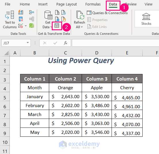
- Go to the Data Tab >> Get & Transform Data Group >> From Table/Range Option.
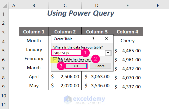
The Create Table wizard will appear.
- Select the data range.
- Click on the My table has headers option.
- Press OK.
The Power Query Editor window will appear.
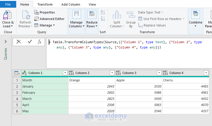
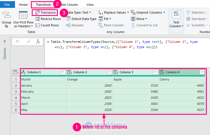
- Select all of the columns of the dataset by pressing CTRL and Left-Clicking on your mouse at the same time.
- Go to the Transform Tab >> Transpose Option.
We can make the first row of our dataset the header too.
- Go to the Transform Tab >> Use First Row as Headers Group >> Use First Row as Headers Option.
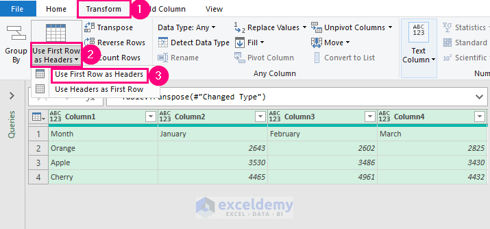
We get the transformed columns from the rows of the main dataset.
- To close this window, go to the Home Tab >> Close & Load Group >> Close & Load Option.
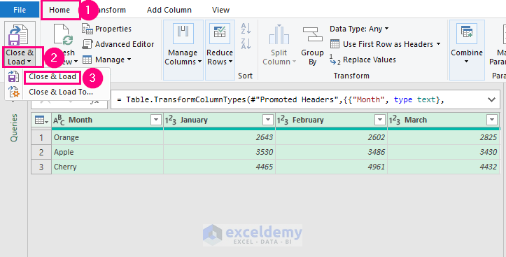
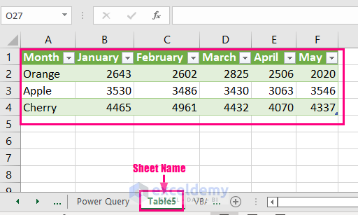
The table in the Power Query Editor window will be loaded to a new sheet named Table5.
Method 8 – Using VBA Code
We can use a VBA code to convert multiple rows into columns.
Steps:
- Go to the Developer Tab >> Visual Basic Option.
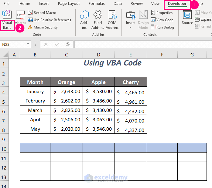
The Visual Basic Editor will open up.
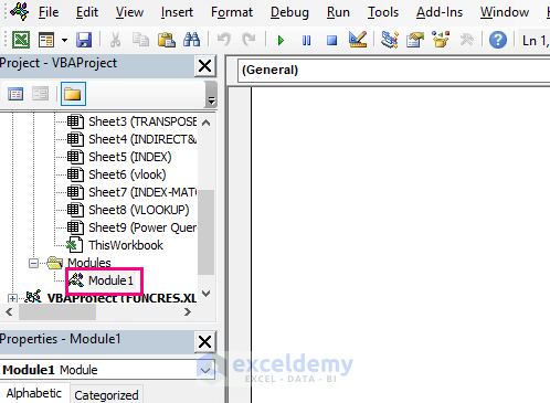
- Go to the Insert Tab >> Module Option.
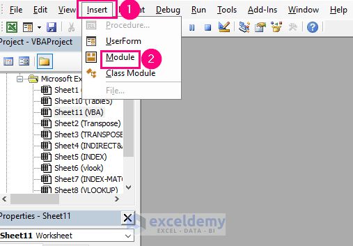
A Module will be created.
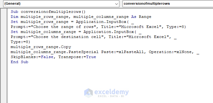
- Enter the following code:
Sub conversionofmultiplerows()

Dim multiple_rows_range, multiple_columns_range As Range
Set multiple_rows_range = Application.InputBox( _
Prompt:="Choose the range of rows", Title:="Microsoft Excel", Type:=8)
Set multiple_columns_range = Application.InputBox( _
Prompt:="Choose the destination cell", Title:="Microsoft Excel", _
Type:=8)
multiple_rows_range.Copy
multiple_columns_range.PasteSpecial Paste:=xlPasteAll, Operation:=xlNone, _
SkipBlanks:=False, Transpose:=True

End Sub
Here, we have declared multiple_rows_range, and multiple_columns_range as Range, and they are set to the range which we will select through the Input Boxes by using the InputBox method.
Then, we will copy the main dataset multiple_rows_range and paste it as transposed in the destination cell multiple_columns_range.
- Press F5.
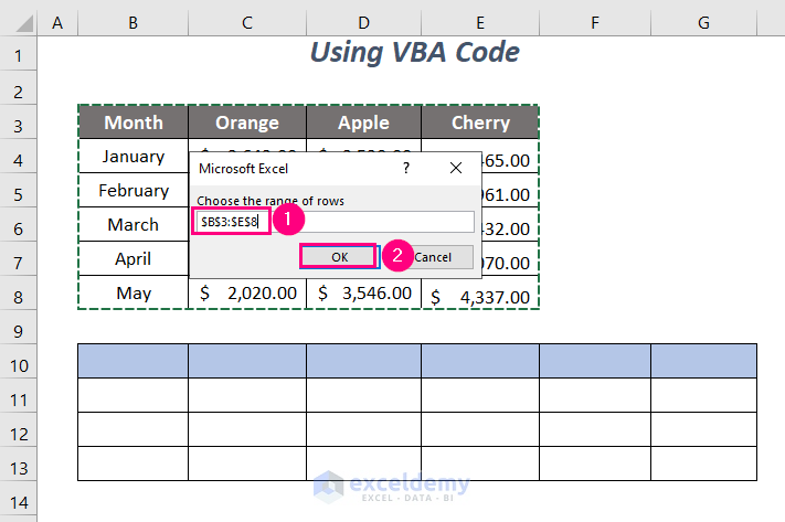
An input box will pop up.
- Select the range of the dataset $B$3:$E$8 in the Choose the range of rows box and press OK.
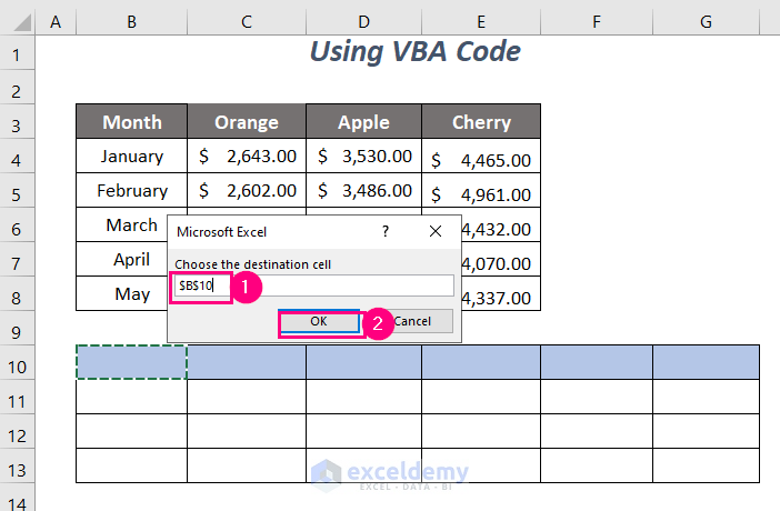
Another input box will pop up.
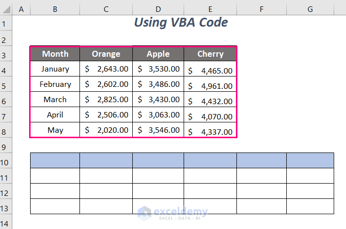
- Select the destination cell $B$10 where you want to have the transposed dataset and press OK.
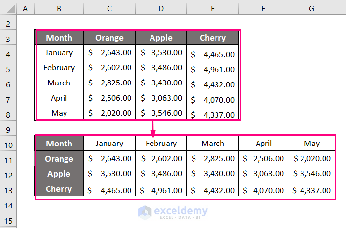
We get the transformed columns, even including the formatting of the main dataset.
Read More: VBA to Transpose Multiple Columns into Rows in Excel
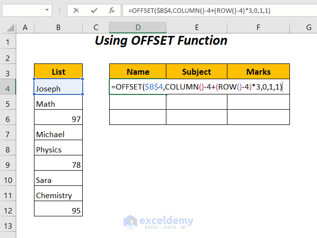
Method 9 – Using the OFFSET Function
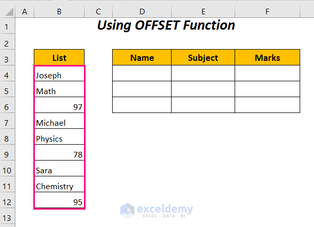
Say we have a list containing some students’ names, their subjects, and corresponding marks in multiple rows. Now, we want to convert the first three rows into three different columns of the table next to this list. Similarly, we want to convert the rest of the rows as columns per three rows. So, we need to convert rows into columns and rows at the same time.
To do this, we are going to use the OFFSET, ROW, and COLUMN functions.
Steps:
- Enter the following formula in cell D4:
=OFFSET($B$4,COLUMN()-4+(ROW()-4)*3,0,1,1)Here, $B$4 is the starting cell of the list.
COLUMN()→returns the column number of cellD4where the formula is being applied.
Output →4
COLUMN()-4becomes
4-4 → 4is subtracted because the starting cell of the formula is inColumn 4
Output →0
ROW() →returns the row number of cellD4where the formula is being applied.
Output →4
(ROW()-4)*3becomes
(4-4)*3 → 4is subtracted because the starting cell of the formula is inRow 4and multiplied with3as we want to transform3rows into columns each time.
Output →0
OFFSET($B$4,COLUMN()-4+(ROW()-4)*3,0,1,1)becomes
OFFSET($B$4,0+0,0,1,1)
OFFSET($B$4,0,0,1,1) → OFFSETwill extract the range with a height and width of1starting from cell$B$4
Output→ Joseph
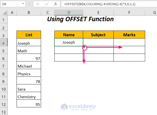
- Press ENTER.
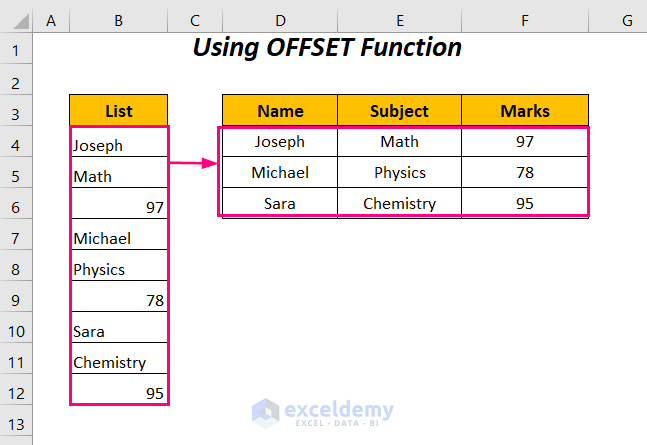
- Drag the Fill Handle tool to the right side and down.
The conversion from multiple rows to columns and rows takes place.
Read More: How to Change Vertical Column to Horizontal in Excel
Download Practice Workbook
Related Articles
<< Go Back to Transpose Data in Excel | Learn Excel
Get FREE Advanced Excel Exercises with Solutions!
