How to Switch Rows and Columns in Excel (5 Methods)

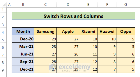
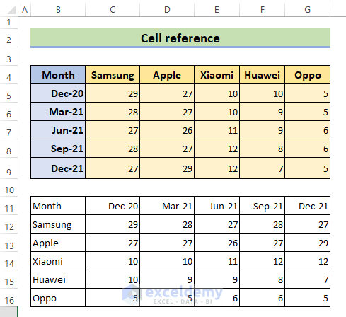
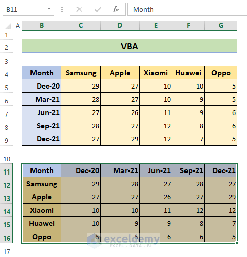
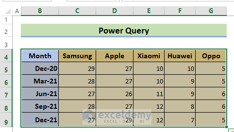
The dataset below shows the market share of smartphone companies.

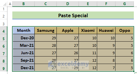
Method 1 – Using the Paste Special (Transpose)

Steps:

• Select the range of cells B4:G9 and press Ctrl+C.

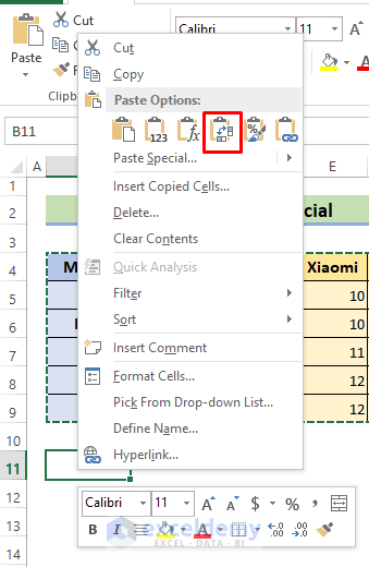
• Right-click over the top-left cell where you want to paste the transposed table. (We chose cell B11, then clicked Transpose.)

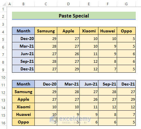
• The data is now switched.

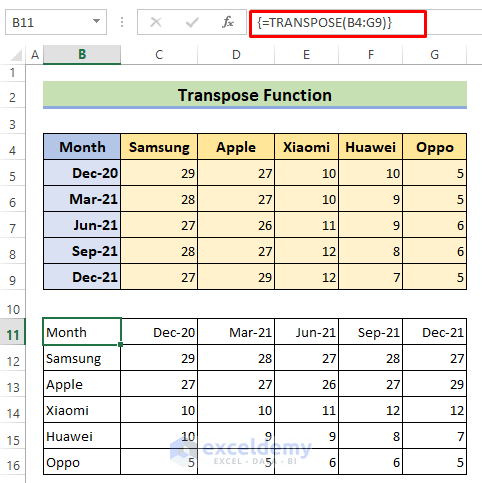
Method 2 – Using the Transpose Function 

Steps:

• Select cell range B11:G16. In the formula bar, type the following formula:

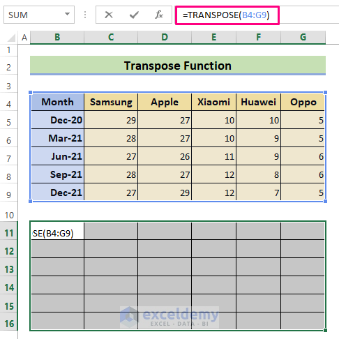
• Press Ctrl+Shift+Enter. The data is now switched.

Notes:

• The transposed data is still linked to the original data. Whenever you change the original data, it will be reflected in the transposed data.
• If you have a current version of Microsoft 365, you can input the formula in the top left cell of the output range and press ENTER to confirm it as a dynamic array formula. Otherwise, use Ctrl+Shift+Enter.

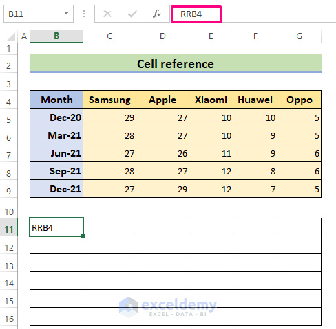
Method 3 – Using Cell Reference 

Steps:

• Select an empty cell (e.g., B11).
• Enter a reference prefix, say ‘RR,’ and the location of the first cell we want to transpose, B4.

• Enter the same prefix ‘RR’ in cell B12 in the cell to the right of the one we used in the previous step. (i.e.,C4, which we’ll type in as RRC4.)
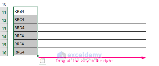
• Continue to enter the references in the cells below.

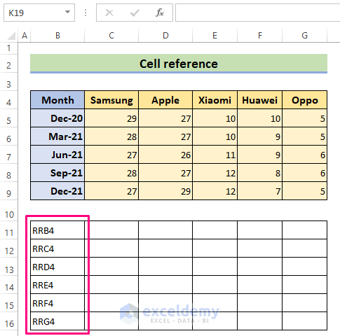
• Select the range of cells B11:B16. Fill the rest of the cells by dragging the Autofill horizontally to Column G.

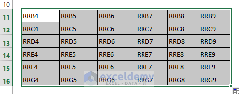
The rest of the cells should be auto-filled.

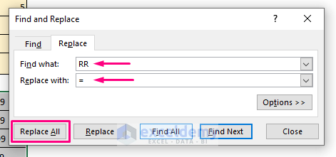
• Press Ctrl+H to bring up Find and Replace. Enter prefix RR into Find what and (=) into Replace with. Click Replace All.

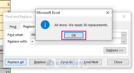
• A pop-up will show “All done. We made 36 replacements.” Click OK.

The data is switched.

Read More: Excel VBA: Get Row and Column Number from Cell Address

Method 4 – Using VBA Macros 

Steps:

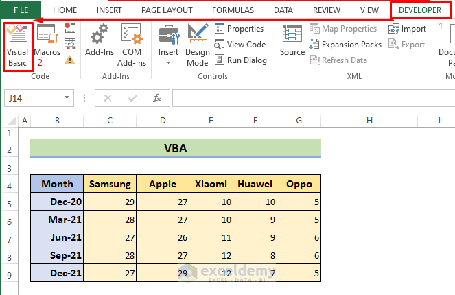
• Go to the Developer tab > Visual Basic.

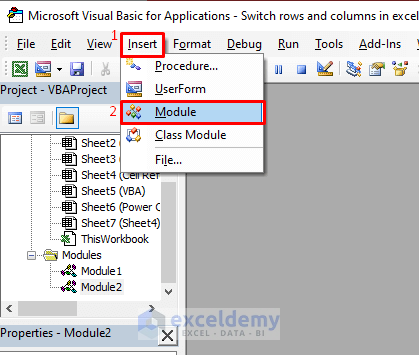
• In the Visual Basic Editor, go to Insert > Module.

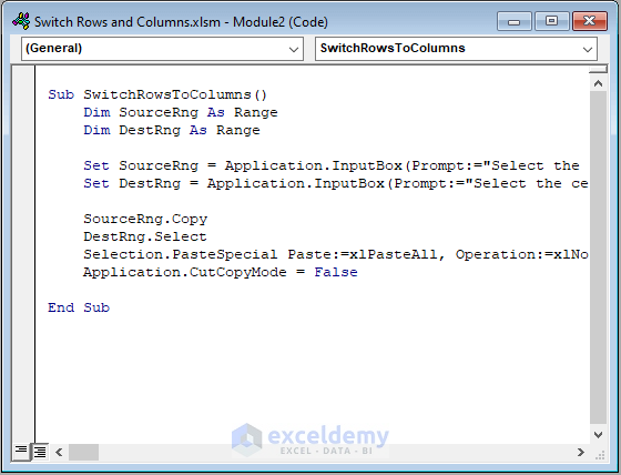
A new module will pop up. Copy the following script:

Sub SwitchRowsToColumns()
    Dim SourceRng As Range
    Dim DestRng As Range
 
    Set SourceRng = Application.InputBox(Prompt:="Select the array to rotate", Title:="Switch Rows to Columns", Type:=8)
    Set DestRng = Application.InputBox(Prompt:="Select the cell to insert the rotated columns", Title:="Switch Rows to Columns", Type:=8)
 
    SourceRng.Copy
    DestRng.Select
    Selection.PasteSpecial Paste:=xlPasteAll, Operation:=xlNone, SkipBlanks:=False, Transpose:=True
    Application.CutCopyMode = False
 
End Sub

• Paste the script into the window and press Ctrl+S to save.

• Close the Visual Basic Editor. Go to Developer > Macros, and you’ll see your SwitchRowsToColumns macro. Click Run.

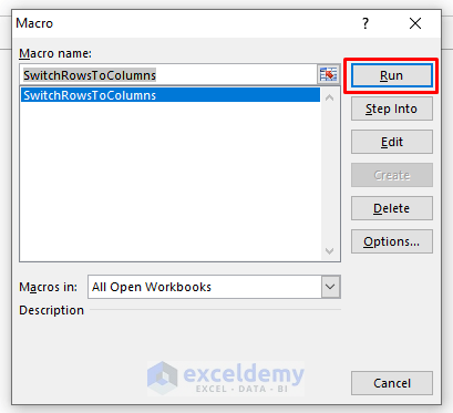
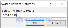
A Switch Rows to Column window will pop up, asking to select the array.

• Select the array B4:G9 to rotate. Click OK.

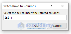
The pop-up will ask you to select the first to insert the rotating columns.

• Select Cell B11. Click OK.

The data is switched.

Read More: Excel VBA to Set Range Using Row and Column Numbers

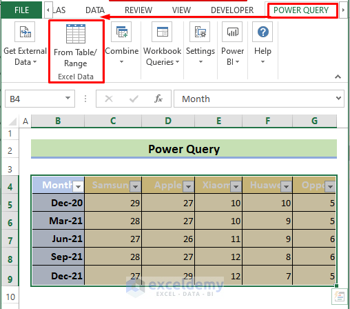
Method 5 – Using Power Query

Steps:

• Select the range of cells B4:G9 to convert rows to columns in Excel.

• Go to the Power Query tab and select From Table/Range.

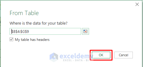
A pop-up will ask the range. Click OK.

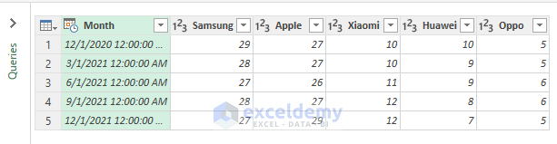
The following table will appear in the Power Query Editor.

• In the Power Query Editor > Go to Transform tab > Select Use First Row as Headers > Select Use Headers as First Row

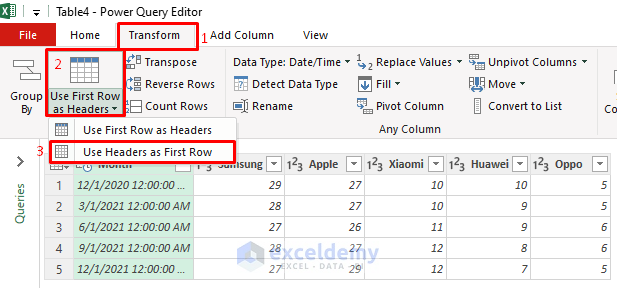
• Click on Transpose under the Transform tab.

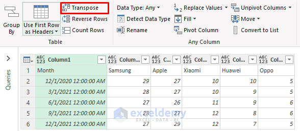
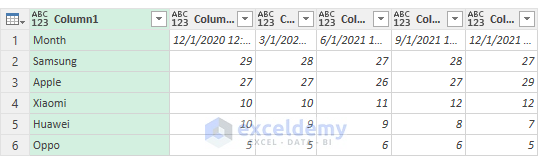
The data is switched.

How to Fix Issues With Transposing Rows and Columns

Overlap Error

If you try to paste the transposed range into the area of the copied range, an overlap error will occur. Choose a cell that is not in the copied range of cells.

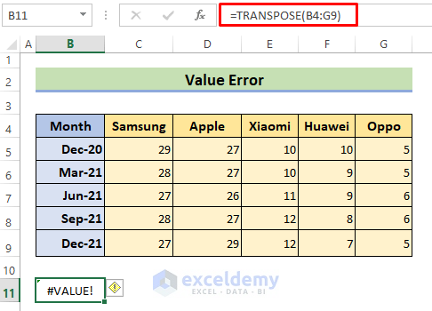
#VALUE! Error

If you implement the TRANSPOSE formula in Excel by pressing Enter, you may see this #VALUE! Error. To avoid this, Press Ctrl+Shift+Enter.

Note: If you have a current version of Microsoft 365, you can input the formula in the top-left cell of the output range and press Enter to confirm it as a dynamic array formula. In older versions, the formula must be entered as a legacy array formula by first selecting the output range, inputting the formula in the top-left cell of the output range, and then pressing Ctrl+Shift+Enter to confirm it.

Read More: [Fixed!] Rows and Columns Are Both Numbers in Excel

Download the Practice Workbook

You can download the workbook to practice.

Further Readings

• How to Add Rows and Columns in Excel
• How to Find Difference Between Rows and Columns in Excel
• How to Lock Column Width and Row Height in Excel
• [Fixed!] Missing Row Numbers and Column Letters in Excel

<< Go Back to Rows and Columns in Excel | Learn Excel