How to Lock Column Width and Row Height in Excel (3 Suitable Ways)

While working with Microsoft Excel, we might have to block a user from modifying the cell height and width. Locking the width of a column or the height of a row limits modifications to the structure. In this article, we will demonstrate how to lock column width and row height in Excel.

How to Lock Column Width and Row Height in Excel: 3 Easy Ways

If we want each segment to be the same, locking the width and height of a worksheet layout might help to accomplish the work. Locking the cell sizes gives the spreadsheet a more uniform visual appearance, which enhances the data’s formal impression. When utilizing worksheet templates, a standard layout may help you stay organized and produce a more appealing end output.

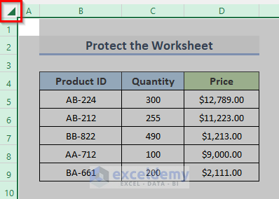
To lock column width and row height, we are going to use the following dataset. The dataset contains some Product IDs in column B, the Quantity of available products in column C, and the Price of each product in column D.

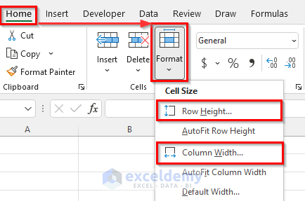
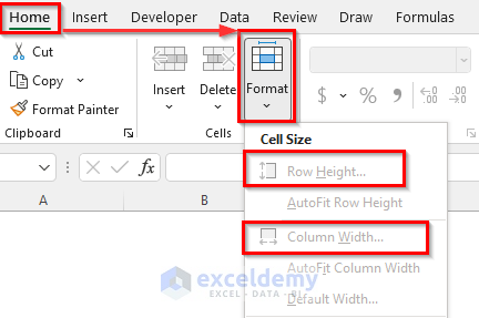
We can format the row height and column width as per our requirements by going to the Home tab > Format drop-down menu on the ribbon.

Let’s look at the ways to lock column width and row height in the following sections.

1. Protect Worksheet to Lock Column Width and Row Height

We can lock column width and row height by protecting the workbook. For this, we need to follow some procedures.

Step 1: Disable Locked Option from Format Cells Feature

To disable the locked option from format cells we need to follow some sub-procedure.

• Firstly, click on the tiny triangle in the upper left corner of the worksheet to select the whole worksheet.

• Secondly, right-click on the worksheet and click on Format Cells.

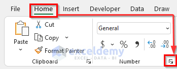
• Alternatively, go to the Home tab from the ribbon and click on the tiny Number Format icon under the Number group.

• This will open the Format Cells dialog box.
• Now, go to the Protection menu and uncheck the Locked option.
• After that, click on the OK button.

• After disabling the locked option now we need to protect our worksheet.

Step 2: Apply ‘Protect Sheet’ Option from Review Tab

To apply the protect sheet option from the review tab we have to follow some sub-steps down.

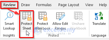
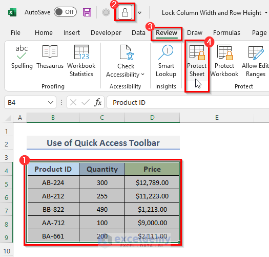
• In the first place, go to the Review tab from the ribbon.
• Then, under the Protect category, click on Protect Sheet.

• This will launch the Protect Sheet.
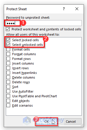
• Now, in the Password to unprotect sheet box, type your password to lock the worksheet. And check-mark the Select locked cells and Select unlocked cells.
• Then, click OK.

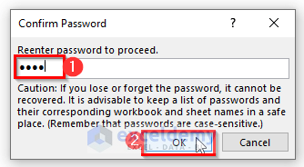
• Further, to confirm the password input the same password again in the Reenter password to proceed.
• Then, click OK.

• Finally, this will lock the column width and row height of your entire workbook. If you go to the Home tab and click on the Format drop-down menu, you can’t change the Row Height and Column Width from the Cell Size menu bar.

2. Insert Quick Access Toolbar to Lock Column Width and Row Height of Cells

We can lock cells’ column width and row height by using the Quick Access Toolbar (QAT). The Quick Access Toolbar (QAT) is a component of Microsoft Excel that provides a list of specific or frequently used controls that may be used and created in any scenario. To lock column width and row height of cells we need to follow some procedures down.

Step 1: Enable Lock Cell from QAT

Let’s follow some sub-procedures to enable the locked cell from the Quick Access Toolbar.

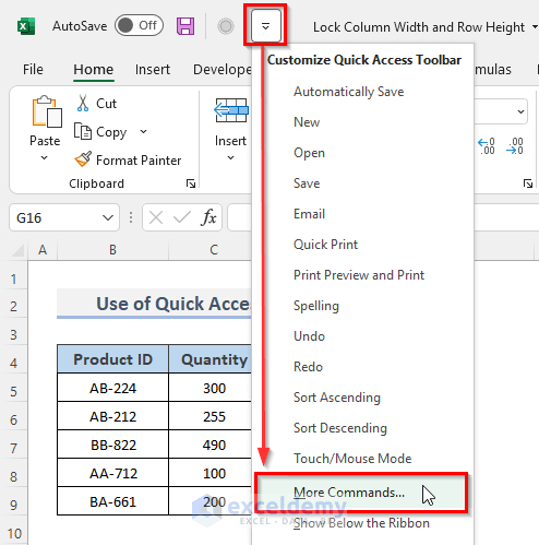
• To begin with, click on the small icon on the top of the excel ribbon.
• Then, click on More Commands to open the Excel Options dialog.

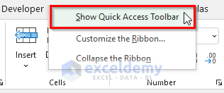
NOTE: The QAT appears in the top left-hand corner of an Excel spreadsheet as usual, and it can be shown farther from the ribbon. But if you can’t find the option, just right-click on the toolbar and click ok Show Quick Access Toolbar. This will allow you to show the QAT menu on the top left-hand corner of the excel file.

• Or, to open the Excel Options dialog, you can go to the File tab from the ribbon.

• Next, click on Options.

• This will launch the Excel Options screen.
• Furthermore, go to the Quick Access Toolbar, and choose All Commands from Choose commands from the drop-down menu.
• And, click on the Lock Cell to add it to the Compare and Merge Workbooks.
• Next, click on Add, and you can see the Lock Cell is now added to the Compare and Merge Workbooks.
• Lastly, click OK to close the Excel Options dialog.

• This will add the Lock Cell option on the top left-hand corner of the workbook.

Step 2: Protect Worksheet to Lock Cells

Now, we need to protect the worksheet to lock the cells. For this let’s look at the sub-steps below.

• Select the entire dataset and click on the Lock option on the top-of-the excel ribbon.
• Further, go to the Review tab and click on Protect Sheet under the Protect category.

• This will open the Protect Sheet dialog screen.
• Now, to lock the worksheet, put your password in the Password to unprotect sheet box. And also, check-mark the Select locked cells and Select unlocked cells.
• Then press OK.

• After that, enter the same password in the Reenter password to proceed field to confirm the password.
• Furthermore, press OK.

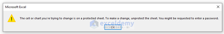
• Finally, the column width and row height of your dataset’s cells will be protected. A Microsoft Excel error notice will display if you try to resize the row and column of certain cells.

Read More: How to Switch Rows and Columns in Excel

3. Excel VBA for Locking Column Width and Row Height of Cells

With Excel VBA, users can easily use the code which acts as excel menus from the ribbon. To use the VBA code to lock column width and row height of cells, let’s follow the procedure down.

Step 1: Launch the VBA Window

• Firstly, go to the Developer tab from the ribbon.
• Secondly, from the Code category, click on Visual Basic to open the Visual Basic Editor. Or press Alt + F11 to open the Visual Basic Editor.

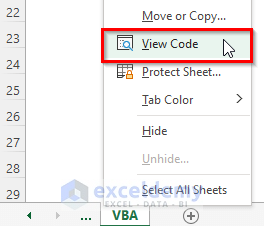
• Instead of doing this, you can just right-click on your worksheet and go to View Code. This will also take you to Visual Basic Editor.

• This will appear in the Visual Basic Editor.
• Thirdly, click on Module from the Insert drop-down menu bar.

• This will create a Module in your workbook.

Step 2: Type & Run the VBA Code

• Copy and paste the VBA code shown below.

VBA Code:

Sub LockingCells()
Dim pwrd As String
Range("B4:D9").Select
Selection.Locked = True
pwrd = InputBox("Enter Password")
ActiveSheet.Protect Password:=pwrd
End Sub

• After that, run the code by clicking on the RubSub button or pressing the keyboard shortcut F5.

Step 3: Enter Password

Now, we need to protect the cells by entering a password.

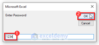
• The earlier steps will appear in a Microsoft Excel pop-up window, asking for inputting the password.
• Now, input your password in the Enter Password field.
• Then, click on OK.

• Finally, this will protect your dataset’s cells’ column width and row height. Here, if you want to resize the row and column of those cells, a Microsoft Excel error message will appear.

Read More: [Fixed!] Missing Row Numbers and Column Letters in Excel

Download Practice Workbook

You can download the workbook and practice with them.

Conclusion

The above methods will assist you in Lock Column Width and Row Height in Excel. Hope this will help you! If you have any questions, suggestions, or feedback please let us know in the comment section.

Related Articles

• Excel Macro: Convert Multiple Rows to Columns
• Excel VBA to Set Range Using Row and Column Numbers
• How to Switch Rows and Columns in Excel Chart
• How to Delete Empty Rows and Columns in Excel VBA
• Excel VBA: Get Row and Column Number from Cell Address
• How to Convert Multiple Rows to Columns in Excel
• [Fixed!] Rows and Columns Are Both Numbers in Excel
• Excel VBA: Set Range by Row and Column Number
• How to Add Rows and Columns in Excel
• How to Find Difference Between Rows and Columns in Excel