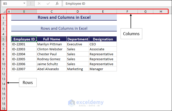
In Microsoft Excel, rows and columns form a grid structure in the spreadsheet. Each cell in the grid is identified by a unique combination of its row number and column letter.
In the following image, the column and row headers are displayed. The intersection of each row and column makes a unique cell.
Excel Rows vs Columns
Here is a table to show the key differences between rows and columns of Excel.
| Particulars | Rows | Columns |
|---|---|---|
| Definition | Horizontal portions of Excel cells | Vertical portions of Excel cells |
| Addressing | Identified by numbers | Identified by letters |
| Size Parameter | Height | Width |
| Total Numbers in a Sheet | 1,048,576 | 16,384 |
| Selection |
|
|
| Direction | Horizontally from left to right | Vertically top to bottom |
| Data Organization | Represents a separate record or entry | Represents a specific attribute or characteristic of the data |
| Example to SUM two Items | =SUM(7:8) | =SUM(C:D) |
| Total Value Display Location | To the bottom | To the right |
| Formatting | Height adjustment, text alignment, and cell borders can be applied to entire rows. | Width adjustment, text alignment, and cell borders can be applied to entire columns. |
| Expanding Data | New rows are inserted above or below existing rows. | New columns are inserted to the left or right of existing columns. |
| Scrolling | Horizontal | Vertical |
How to Navigate Rows and Columns in Excel
Here are two simple keyboard shortcut tips to navigate rows and columns in Excel.
- Press Ctrl + Down Arrow to go to the last row of a data table or the last row of the sheet if there are all empty cells under the data table. To get back to the previous position, press Ctrl + Up Arrow.
- Press Ctrl + Right Arrow to go to the last column of a data table or the last column of the sheet if there are all empty cells to the right of the data table. To get back to the previous position, press Ctrl + Left Arrow.
Here is an image showing how this navigation works.
How to Insert or Delete a Row in Excel
Excel always inserts a new row above another. We can use the Insert and Delete commands to insert or delete a row or multiple rows respectively. The process of adding rows or columns is pretty much the same.
Insert Row or Rows
To insert a new row above another row, you need to select the lower row first.
- Select any cell of the 8th row.
- Right-click on it to open the Context Menu.
- Select Insert.
- Select Entire Row in the Insert dialog box and click OK.
In the image above, you can see that a new row is added at the 8th row. The 8th row becomes the 9th row of the table.
To insert multiple rows, just select multiple cells of the corresponding rows and apply the previous command. Here, we want to insert two rows above the 7th row.
- Select the range B7:B8.
- Use the same steps as above.
You can also insert a row or multiple rows above another using the context menu from the row header.
- Right-click on the row header.
- Select Insert.
Delete Row or Rows
The process of deleting a row or multiple rows is similar to the process of inserting rows. Right-click in the relevant row and select the Delete command from the Context Menu. See the image below.
Here is another image showing the procedure of deleting multiple rows.
How to Insert or Delete a Column in Excel
Excel always inserts a new column to the left of the current column. We can use the Insert and Delete commands to insert or delete a column or multiple columns respectively.
- Select any cell of column C.
- Right-click on it to open the Context Menu.
- Select the Insert option.
- Select Entire Column in the Insert dialog box and click OK.
A new column is added to the left of the Full Name column. Column C becomes Column D.
To insert multiple columns, just select multiple cells of the corresponding columns and apply the previous steps.
- Select the range B7:B8.
- Right-click on it to open the Context Menu.
- Select the Insert option.
- Select Entire Column in the Insert dialog box and click OK.
Note: You can also insert or delete rows or columns from the Insert and Delete drop-down of the Cells group.
Delete Column or Columns
The process of deleting a column or multiple columns is similar to the process of inserting columns. Just right-click on the relevant column select the Delete command from the Context Menu. See the image below.
Here is another image showing multiple columns being deleted.

How to Group Rows and Columns in Excel
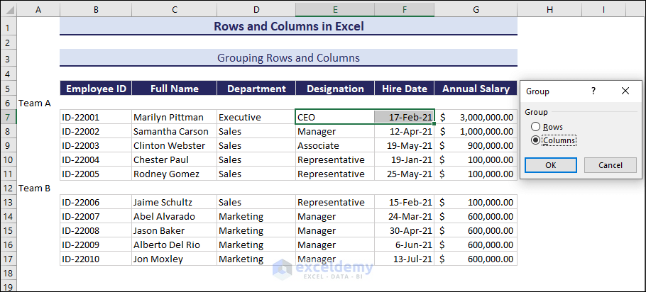
Grouping rows or columns keeps the data in a group. You can view or hide the group at any time. In this example we will group the rows under Team A.
- Select the rows under Team A.
- Select Data >> Outline >> Group.
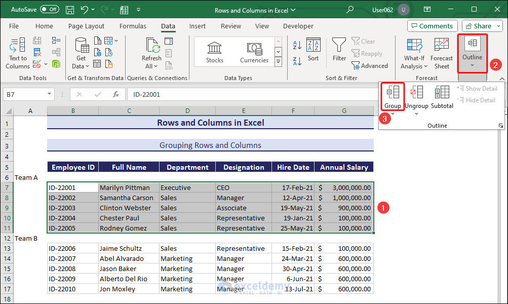
Click on the image to enlarge
- The Group dialog box will appear.
- Select Rows and click OK.
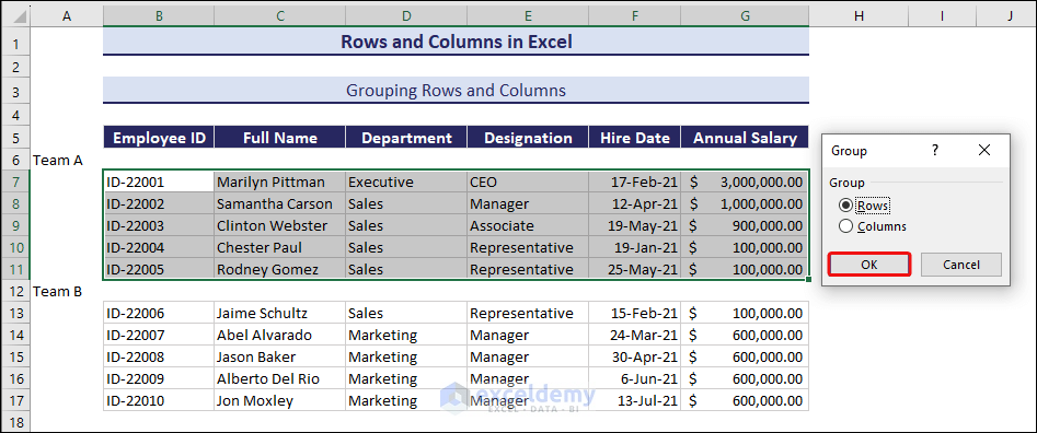
Click on the image to enlarge
Note: You can also open the Group dialog box by pressing Alt + Shift + Right arrow key (→).
The selected rows are now grouped. You can hide them by clicking the Minus (–) button and unhide them by clicking the Plus (+) button. See the image below.
Similarly, you can group columns of a data table.
- Select the cells of the corresponding columns and open the Group dialog box.
- Select Columns and click OK.
Click on the image to enlarge
You can see the Minus button above the column header. Click it to hide the column or columns and click the Plus button to unhide them.
Note: You can see that there’s the Ungroup command under the Outline group. Use it to ungroup the grouped rows or columns.
How to Switch Row to Column and Vice Versa in Excel
You can switch the rows to columns and vice versa by using the Paste Transpose command.
- Press Ctrl + C to copy the data range.
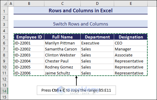
- Right-click on a cell and select Paste >> Transpose command from the Context Menu.
This command will switch the rows to columns and columns to rows.
How to Set Range By Using Row and Column Numbers
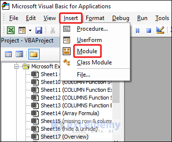
- Open the VBA editor window from Developer >> Visual Basic or press Alt + F11 (Alt + fn + F11 for laptop users).

- Select Insert >> Module to create a VBA Module.
- Insert the code below in the Module.
Sub SetRange()
    Set mn_Rng = Worksheets("set_range").Range(Cells(5, 2), Cells(15, 7))
    mn_Rng.Select
End Sub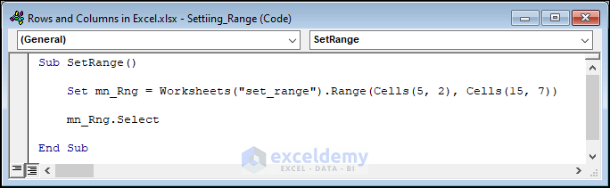
The code sets a range from the (5, 2) cell to the (15, 7) cell which is the range B5:G15. You can apply any value to this range to populate. Here, we have set no value, so the values won’t change in the dataset.
- Go back to the worksheet and select Macros or press Alt + F8 to open the Macros dialog box.
- Run the macro.
You will see that the range B5:G15 are selected.
How to Hide and Unhide Rows and Columns in Excel
To hide a set of rows, we need to select the cells of the corresponding rows and apply the Hide command. Here, we want to hide the 12th and 13th rows.
- Select two cells of these rows. Here, the B12 and B13 are selected.
- Choose Cells >> Format >> Hide & Unhide >> Hide Rows.
Click on the image to enlarge
- To unhide the hidden rows, select the rows above and below to the hidden rows. Here we selected the cells of 11th and 14th rows.
- Use the Unhide Rows command to display the hidden rows.
Click on the image to enlarge
You can hide and unhide columns in the same manner. Here is an image illustrating how to hide columns.
Click on the image to enlarge
And the following image shows how to unhide the hidden columns.
Click on the image to enlarge
How to Lock Column Width and Row Height in Excel
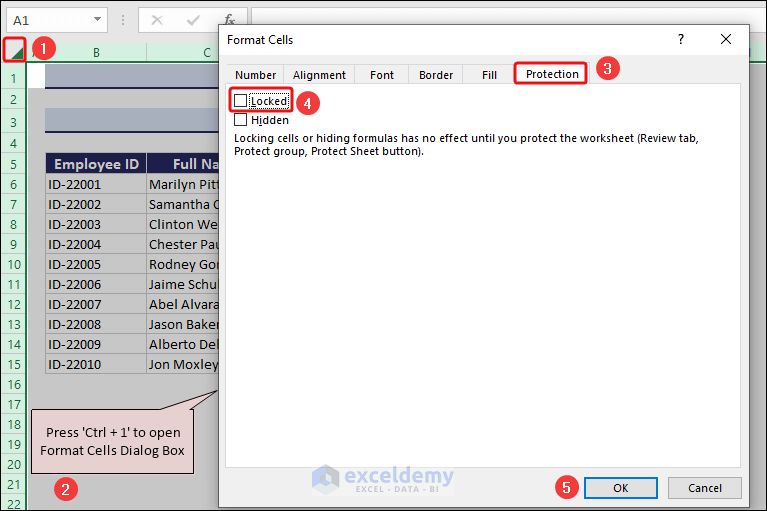
- Select the triangle icon (marked 1 in the image). This will select all the cells in the sheet.
- Press Ctrl + 1 to open the Format Cells dialog box.
- Select the Protection tab >> uncheck the Locked
- Click OK.
- Select Review >> Protect Sheet.
- In the Protect Sheet dialog box, check all the options except Format columns and Format rows.
- Insert a password and click OK.
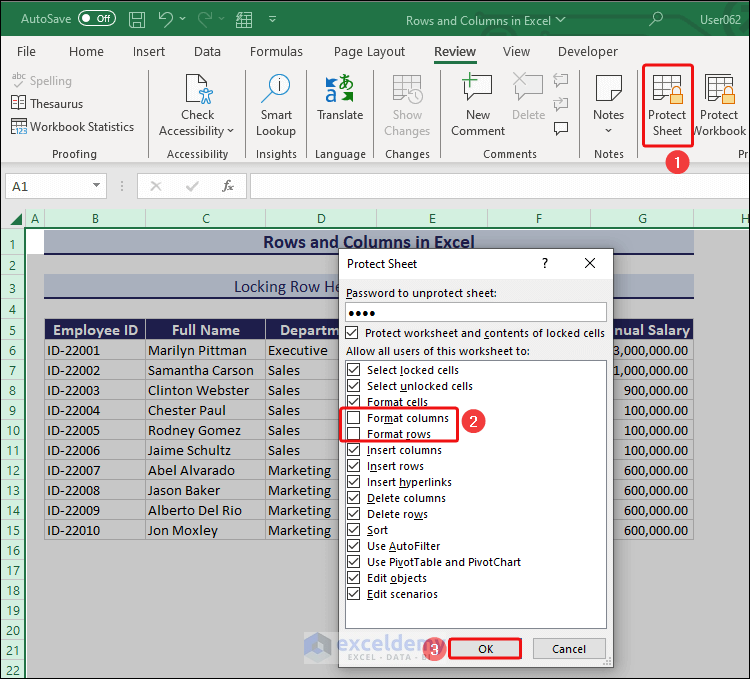
Reenter the password in the next dialog box and click OK.
You can edit a cell or cell content but you cannot edit the column width or row height. The icon for editing the width and height does not appear when the cursor is placed at the row or column header section.
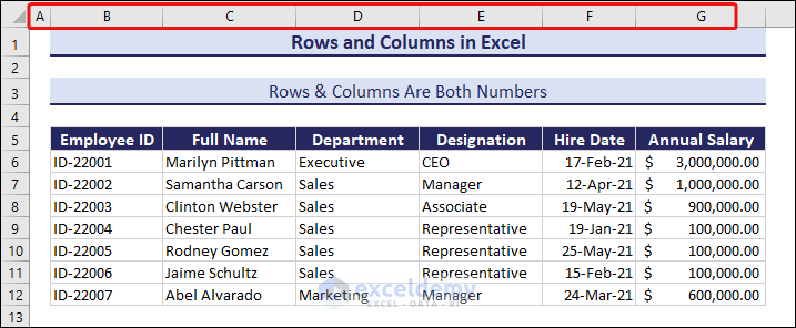
[Issue] Why are My Rows and Columns Both Numbers in Excel
Sometimes, rows and columns can be both numbers due to a change in the settings.
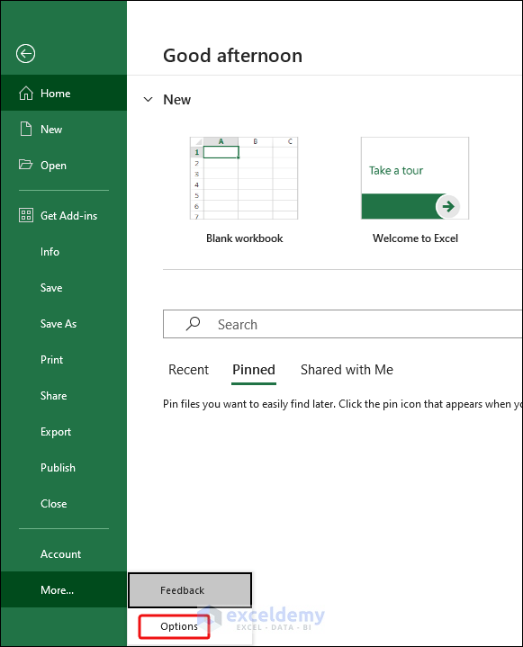
- Open the File tab.
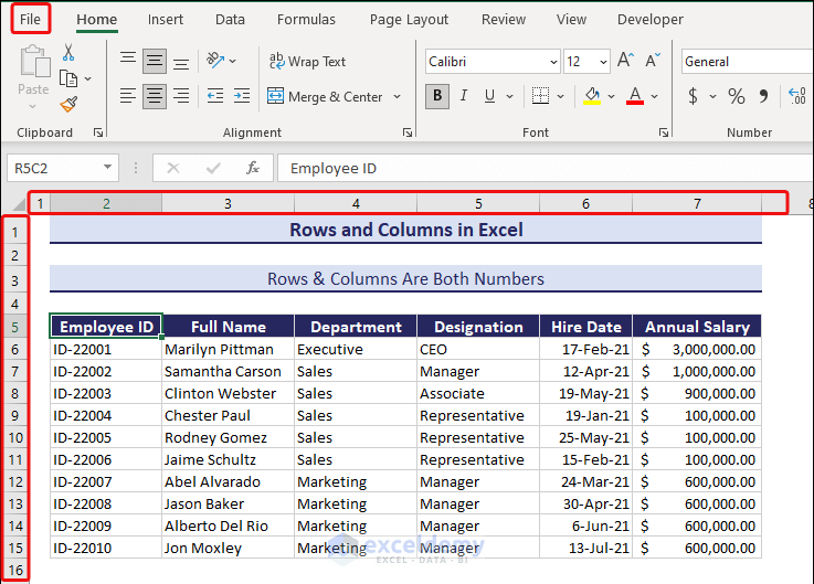
- Open the Options.
- Select Formulas >> uncheck R1C1 reference style and click OK.
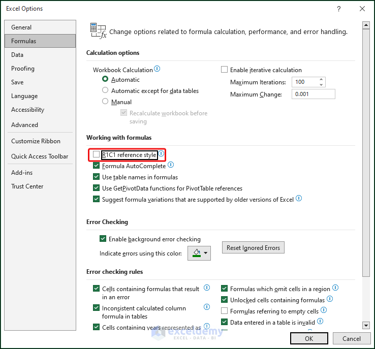
The column letters appear in the column header section.
[Issue] Why Am I Missing Row Numbers and Column Letters in Excel
- Select the View tab.
- Check the Headings in Show.
Rows and Columns in Excel: Knowledge Hub
<< Go Back to Learn Excel
Get FREE Advanced Excel Exercises with Solutions!
