Excel Row and Column Headings – A Guide

This is an overview:

Download Practice Workbook

Download the workbook to practice.

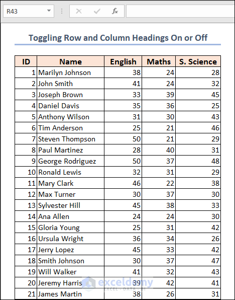
Excel Row and Column Headings

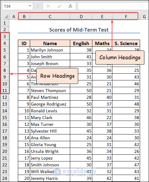
Row and column headings are like labels.

Row headings are the numbers on the left side of the worksheet. Each row has its own number: 1, 2, 3, and so on. These numbers help identify and locate specific rows.

Column headings are the letters at the top of the worksheet. They start with “A” and go in alphabetical order as you move to the right.

Cell Reference Styles with Row and Column Headings in Excel

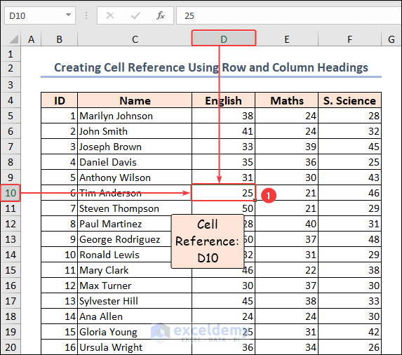
To create a cell reference, combine the column letter and the row number of a cell.

• 25 was selected and highlighted in the following image. This cell refers to Column D and Row 10. The cell reference is D10. You can see the cell reference in the Name Box at the left top corner.

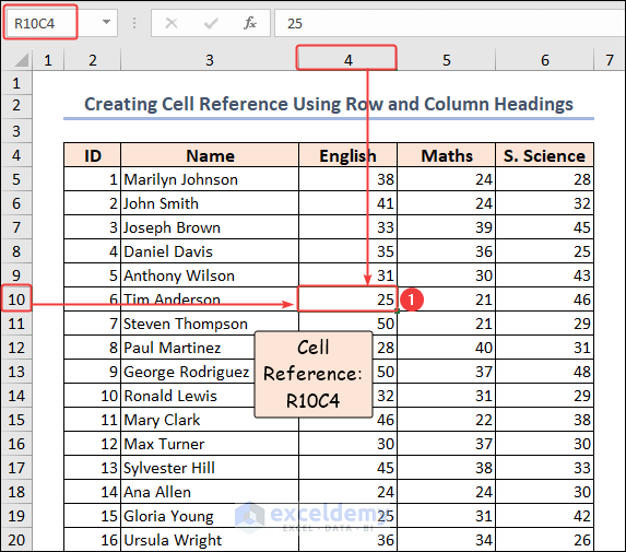
In the R1C1 reference style, the row number is followed by the column number.

• Select the same cell. It is positioned in Row 10 and Column 4. The cell reference becomes R10C4.

Toggling Row and Column Headings On or Off in Excel

You can hide and unhide the headings.

• Go to the View tab and uncheck Headings.

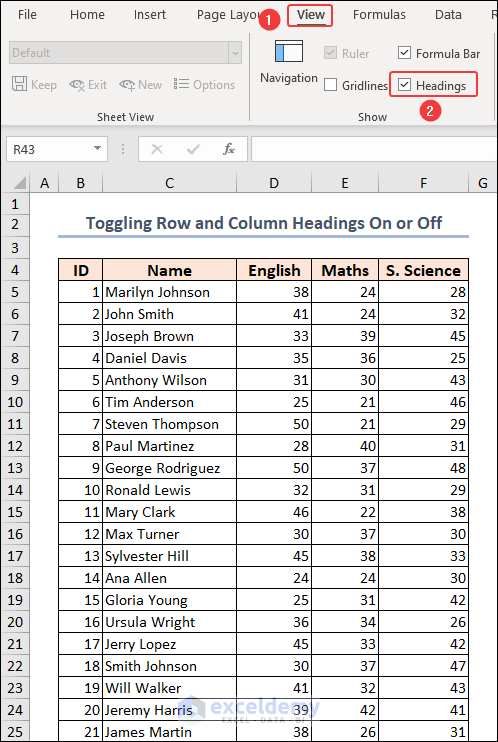
The headings are not shown.

Check the Headings to display them.

Read More: How to Rename Column in Excel

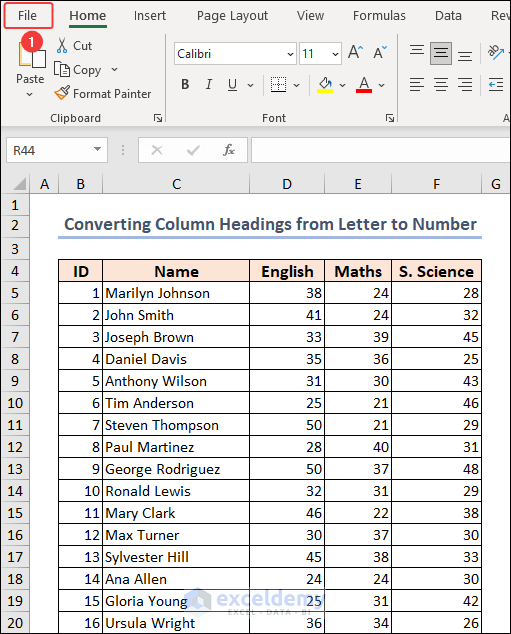
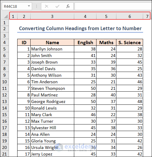
Convert Column Headers from Letters to Numbers and Vice Versa

• Go to the File tab.

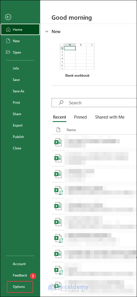
• Click Options.

• In the Excel Options dialog box, go to Formulas.
• Check R1C1 reference style in Working with formulas and click OK.

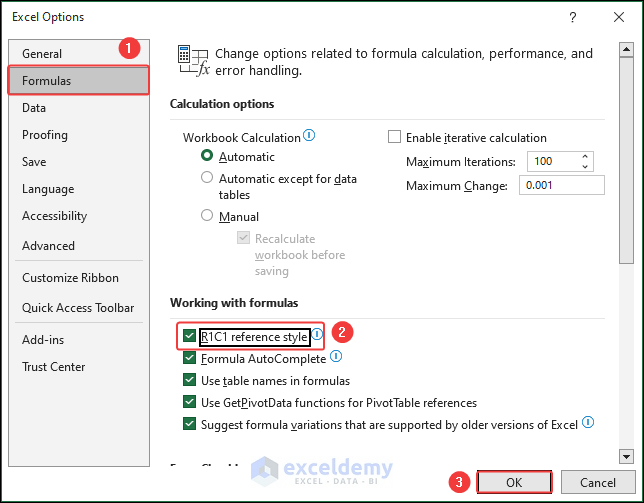
The letters are converted to numbers.

Uncheck R1C1 reference style to undo.

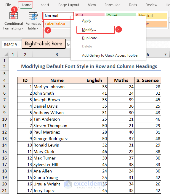
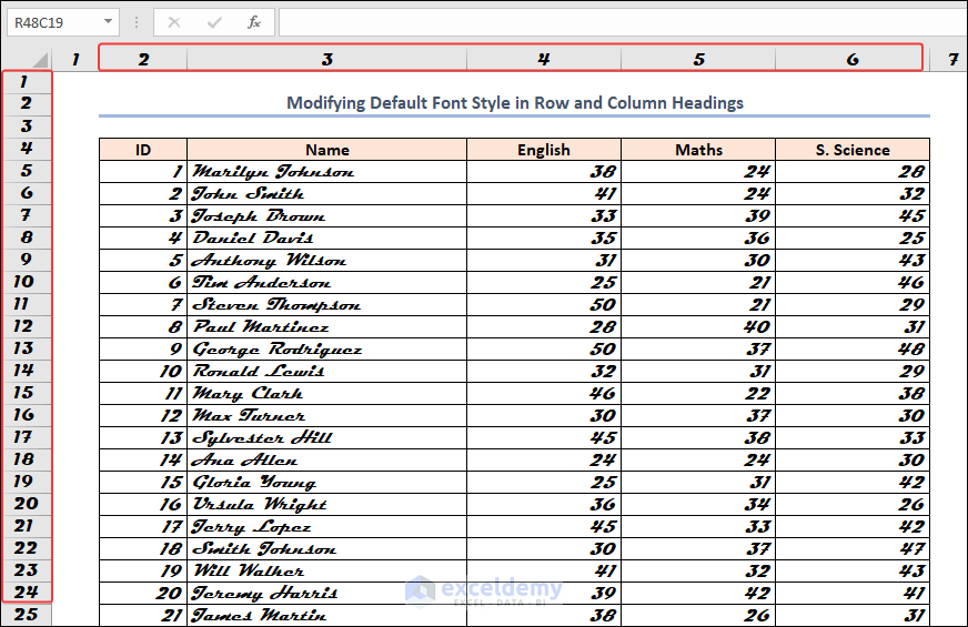
Modify the Default Font Style in Row and Column Headings in Excel

• Go to the Home tab.
• Right-click Normal in Style.
• Click Modify….

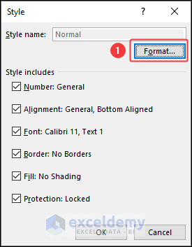
• Click Format in the Style dialog box.

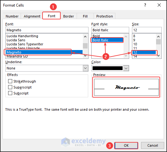
• In the Format Cells dialog box, go to the Font tab.
• Select Font and choose a Font style.
• Click OK.

• Click OK in the Style dialog box.

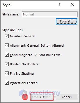
The default font changes.

Read More: How to Title a Column in Excel

Print Row and Column Headings in Excel

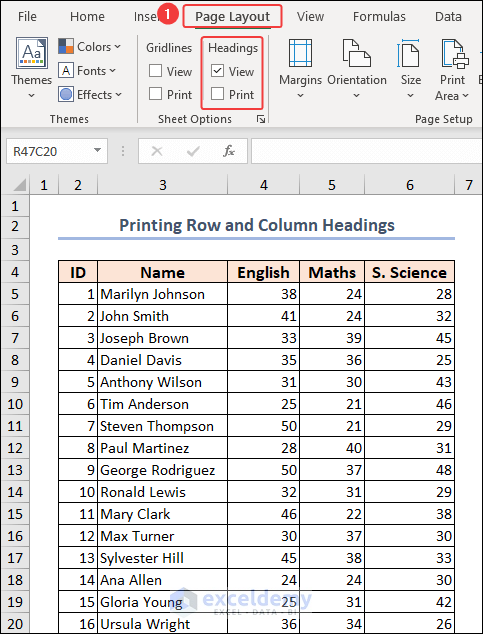
• Go to the Page Layout tab.
• In Sheet Options, you can see two options: View and Print. The first one is checked and the second one is unchecked by default.

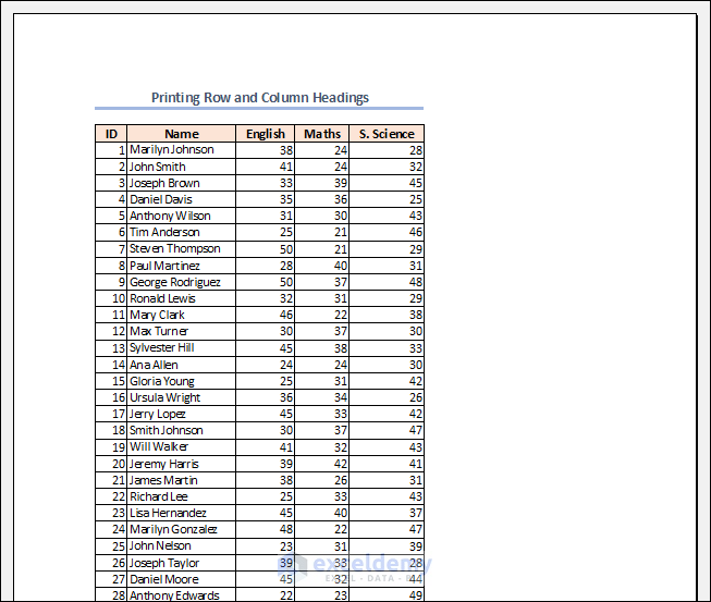
• Press CTRL + P to open the Print options. You can see the Print Preview.

The headings are not visible in the Print Preview:

• In Page Layout, check Print.

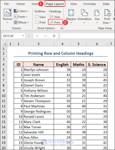
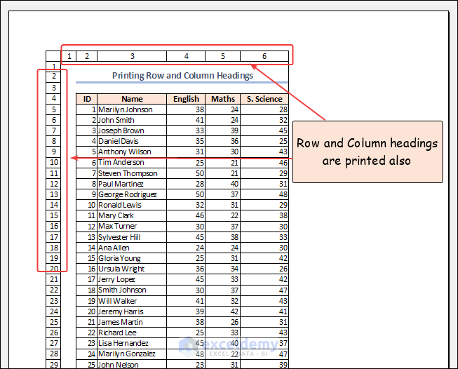
• Press CTRL + P. Row and column headings will be printed.

Read More: Keep Row Headings When Scrolling Without Freeze

How to Establish Top Row as Header Row in Excel

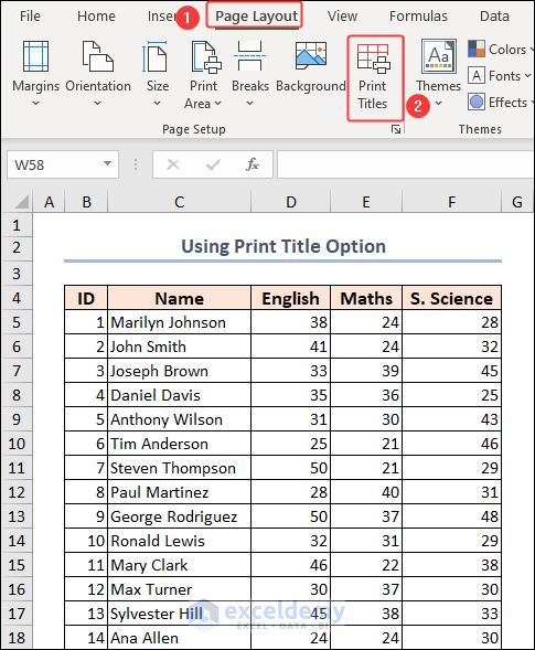
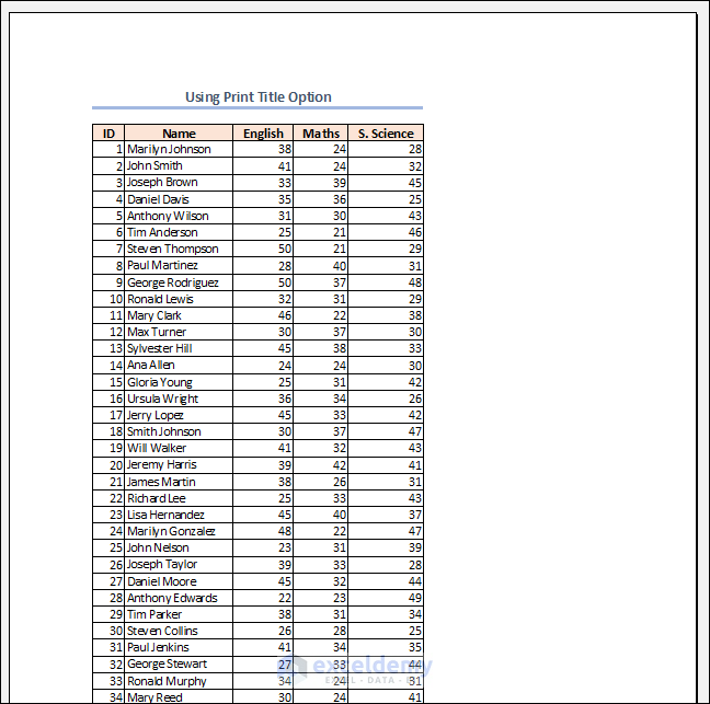
1. Use the Print Title Option

• Click Page Layout >> Print Titles.

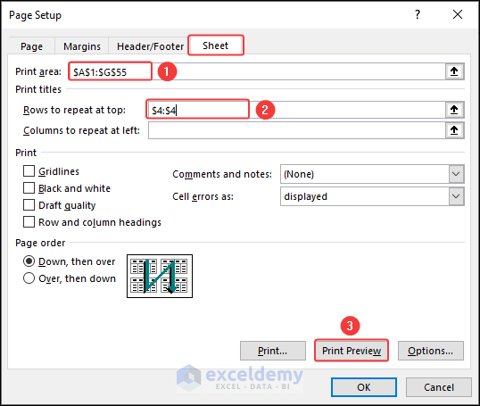
• In the Page Setup dialog box, the Sheet tab is opened by default.
• Enter the cell reference A1:G55 in the Print area and Row 4 in Rows to repeat at top.
• Click Print Preview.

This is the first page.

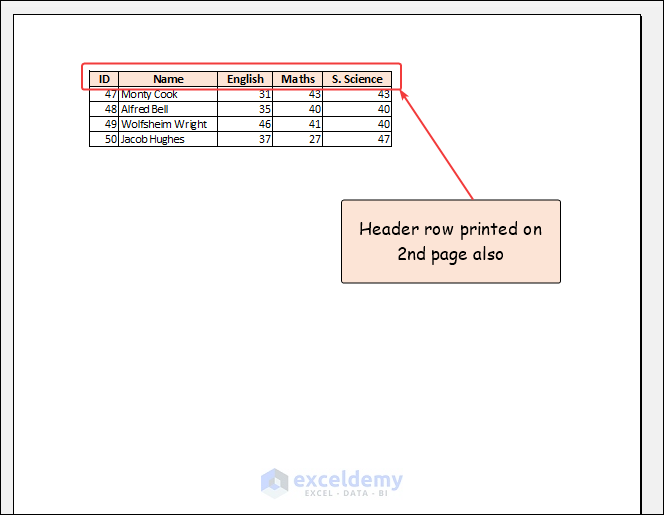
Row 4: the header on the 2nd page is visible.

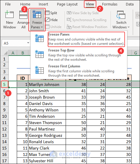
2. Utilize the Freeze Panes

• Click the heading number of Row 5.
• Go to View >> Freeze Panes>> Freeze Panes.

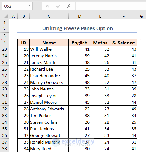
After scrolling down, the header row is displayed.

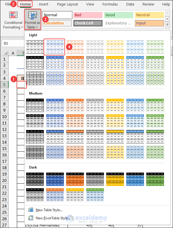
3. Format the Dataset as a Table

• Select B5.
• Go to the Home tab.
• Click Format as Table and choose Light Blue, Table Style Light 2 in Light.

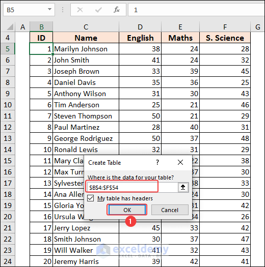
• In the Create Table dialog box, the range is selected automatically.
• Click OK.

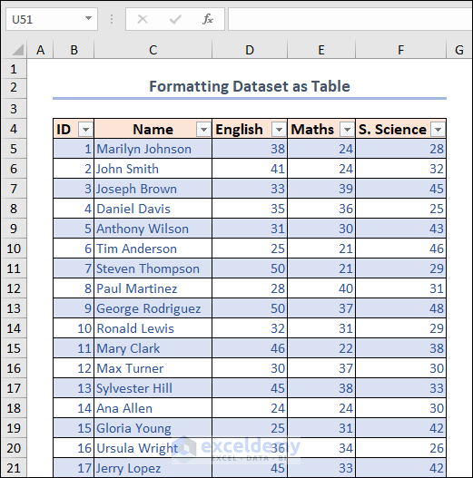
The data range is converted to a table.

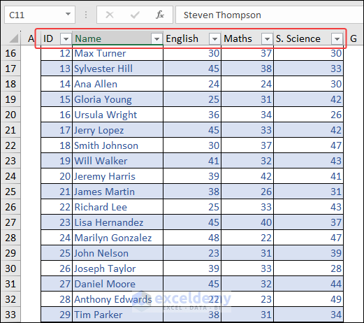
• Click any cell inside the table and go through the worksheet by scrolling down. You can see the headers.

Read More: Create Table with Row and Column Headers

Things to Remember

• The R1C1 reference style in Excel offers several advantages, particularly when working with formulas and writing VBA codes for macros.
• In Excel, the default Font is Calibri 11 pt.

Excel Row and Column Headings: Knowledge Hub

<< Go Back to Rows and Columns in Excel | Learn Excel