How to Title a Column in Excel – 5 Methods

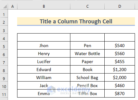
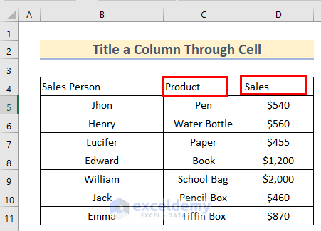
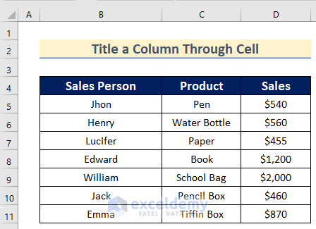
The dataset showcases Sales Person, Product, and Sales.

Method 1 – Title a Column using the Cell in Excel

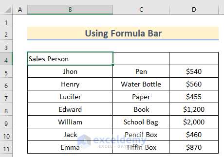
There are blank cells in B4:D4.

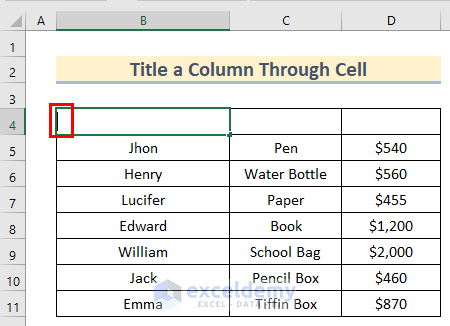
Step1 – Title a Column

• Select B4.
• Double-click the cell.

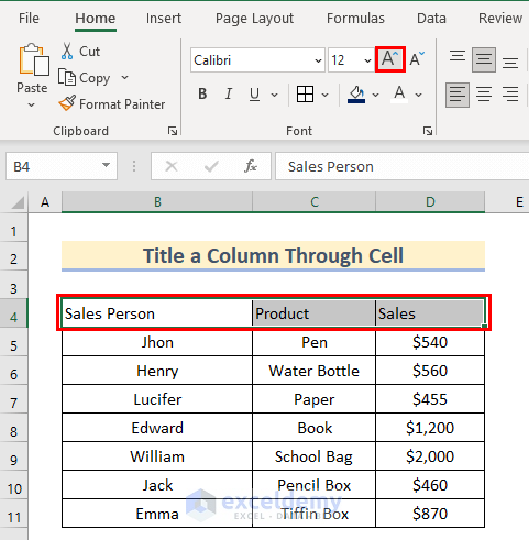
• Enter the title. Here, Sales Person.

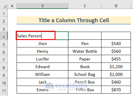
• Press ENTER.

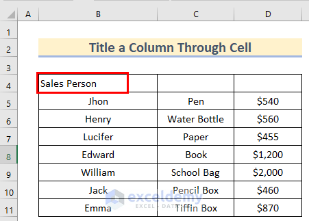
• Add column titles to the rest of the columns. Here, Product in C4 and Sales in D4.

Step 2 – Formatting the Column Title

• Select B4:D4.
• Click Increase Font Size.

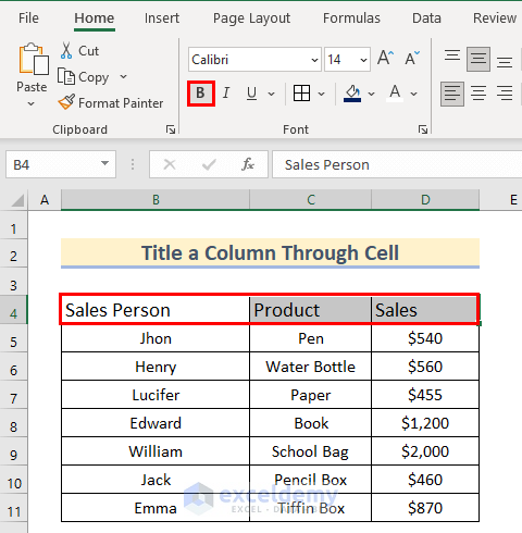
• Click Bold to bold the texts.

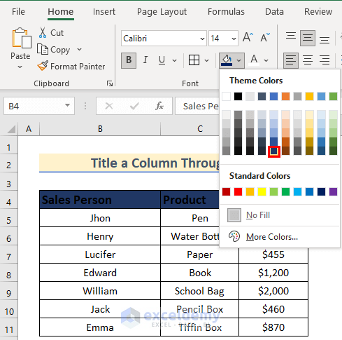
• Click Fill Color to change the color of the cells.

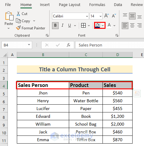
• Select a color. Here, Blue, Accent 1, Darker 50%.

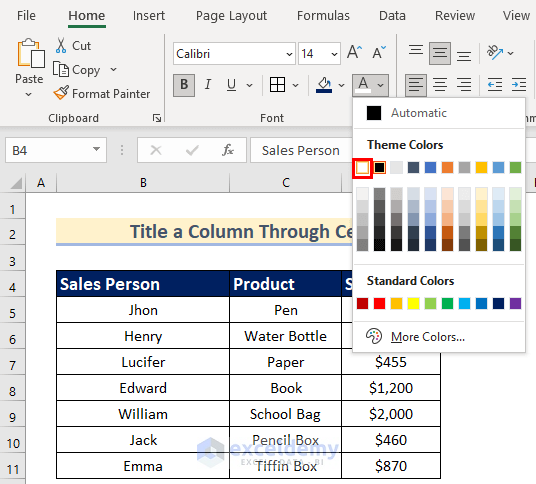
• Click Font Color to change the font.

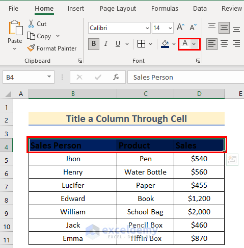
• Select a color. Here, White, Background 1.

• Select Center in Alignment.

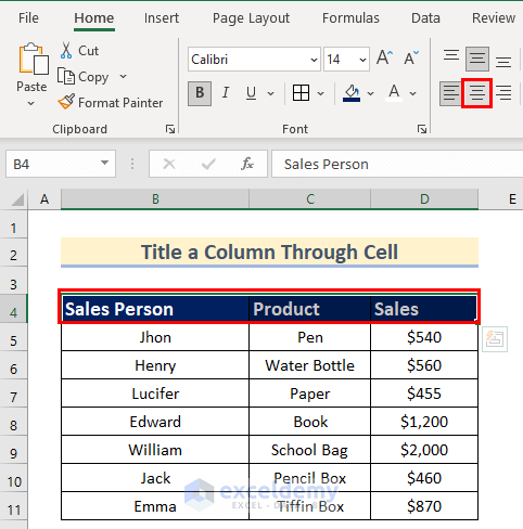
This is the output.

Read More: How to Create Column Headers in Excel

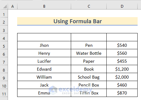
Method 2 – Using the Formula Bar to Title a Column in Excel

Add or change the column headings in B4:D4:

Steps:

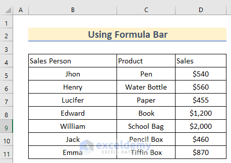
• Select B4.
• Go to the Formula Bar.

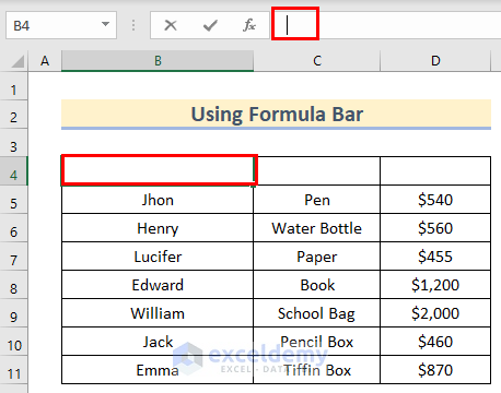
• Enter the column title. Here, Sales Person.

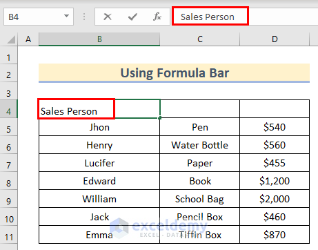
• Press ENTER.

• Add column titles to the rest of the columns. Here, Product in C4 and Sales in D4.

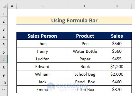
• Format the dataset: follow the steps described in Method 1.

This is the output.

Read More: Remove Column Headers in Excel

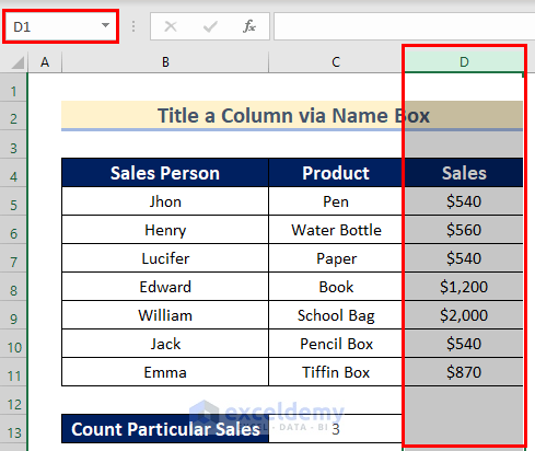
Method 3 – Title a Column using the Excel Name Box

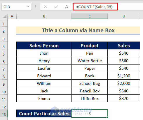
• Enter the following formula in C13.

• Press ENTER.

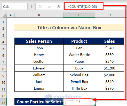
Sales values are counted as $540 in C13.

Steps:

• Select the Entire Column D. You will see D1 in the Name Box.

• Enter Sales as the column name.

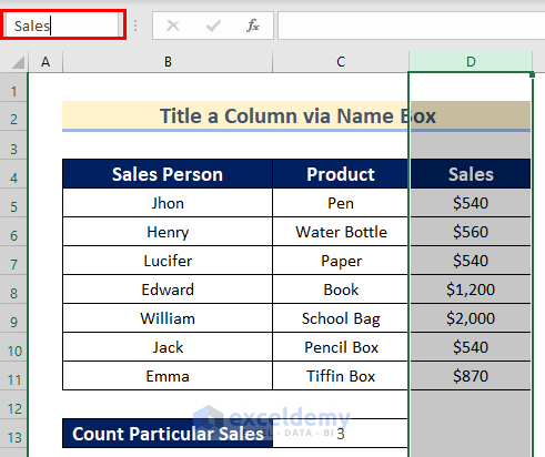
• Press ENTER.

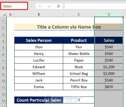
This is the output.

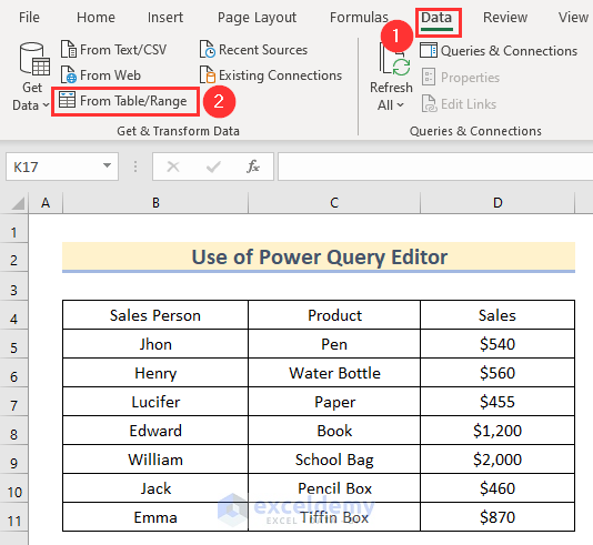
Method 4 – Using the Power Query Editor to Title a Column in Excel

Steps:

• Go to the Data tab >> click From Table/Range.

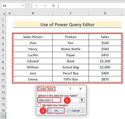
• In Create Table, enter B4:D11.
• Click OK.

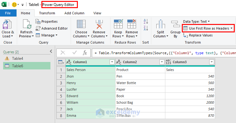
• In the Power Query Editor, click Use First Row as Headers to set the first row as the column title.

• The column titles are selected.

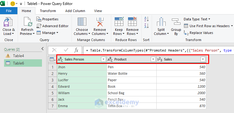
• Click Close & Load >> select Close & Load.

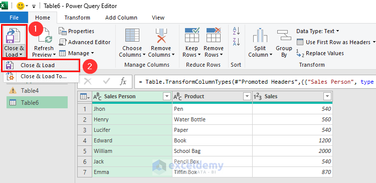
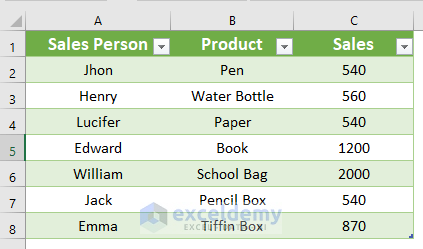
• You will see the column titles.

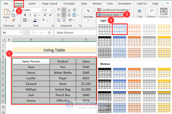
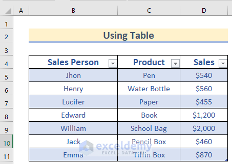
Method 5 – Using a Table to Title a Column

Steps:

• Select B4:D11.
• Go to the Home tab >> click Format as Table >> select Light Blue, Table Style Light 2.

• In Create Table, enter B4:D11.
• Check My table has headers.
• Click OK.

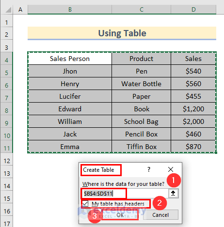
This is the output.

Read More: How to Create Excel Table with Row and Column Headers 

Showing Row Numbers and Column Headers

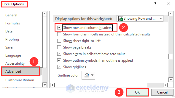
If the row and column headers are hidden:

Steps:

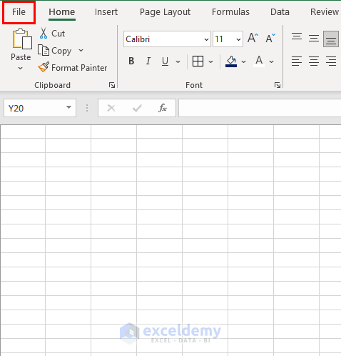
• Go to the File tab.

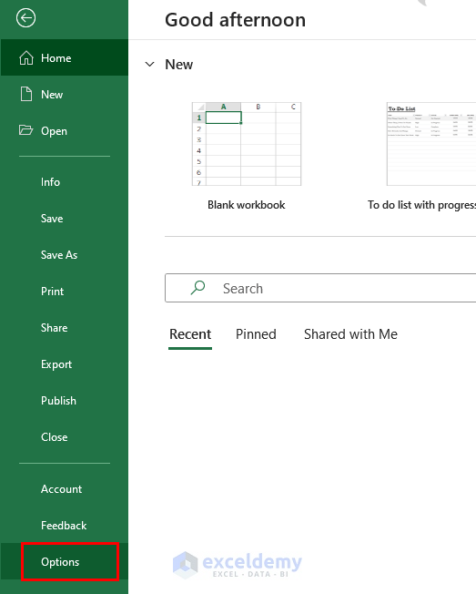
• Click Options.

• In Excel Options, go to the Advanced tab.
• Check Show row and column headers.
• Click OK.

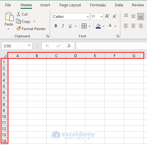
• Row and column headers are displayed.

Download Practice Workbook

Related Articles

• How to Change Excel Column Name from Number to Alphabet
• How to Repeat Column Headings on Each Page in Excel
• How to Remove Column1 and Column2 in Excel
• How to Change Column Header Name in Excel VBA
• [Fixed] Excel Column Numbers Instead of Letters

<< Go Back to Rows and Columns Headings | Rows and Columns in Excel | Learn Excel