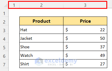
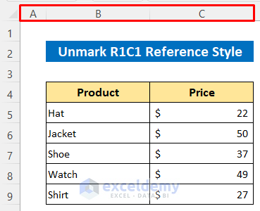
To demonstrate the methods, we’ll use the following dataset representing some products’ prices. The column names are in numerical order.
Method 1 – Unmark R1C1 Reference Style
Steps:
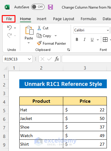
- Click the File option beside the Home tab.
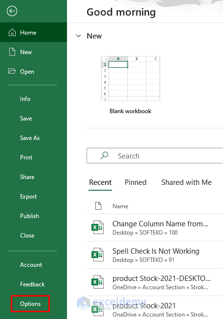
- Click on Options.
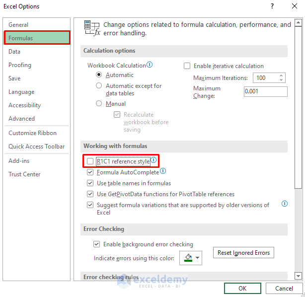
- And a dialog box will open up.
- From the Formulas section, unmark the R1C1 reference style.
- Press OK.
Excel has changed the column name from number to the default alphabet system.
Read More: How to Change Column Header Name in Excel VBA
Method 2 – Use Excel Formula to Convert
2.1 Use the CHAR Function for Single-Letter Columns
Steps:
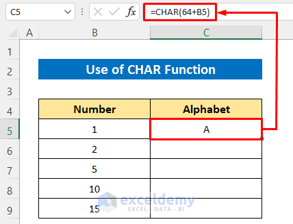
- Enter the following formula in cell C5:
=CHAR(64+B5)- Press the Enter button to get the output.
- Drag the Fill Handle icon to copy the formula for the other cells.
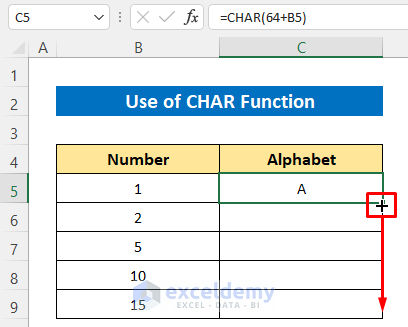
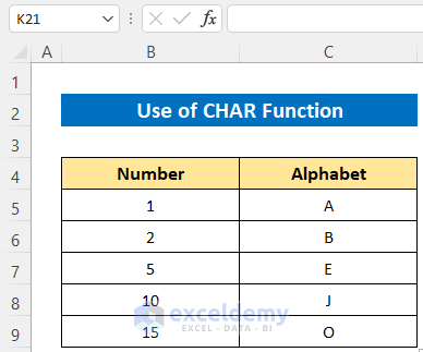
You will get all the column names in alphabetical order.
Read More: [Fixed] Excel Column Numbers Instead of Letters
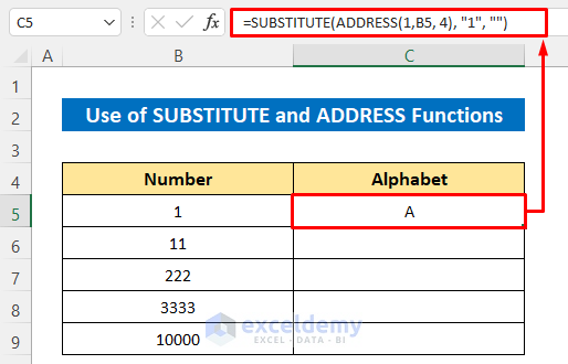
2.2 Use SUBSTITUTE and ADDRESS Functions for Any Column
Steps:
- Enter the following formula in cell C5:
=SUBSTITUTE(ADDRESS(1,B5, 4), "1", "")- Press the Enter button to get the corresponding alphabet.
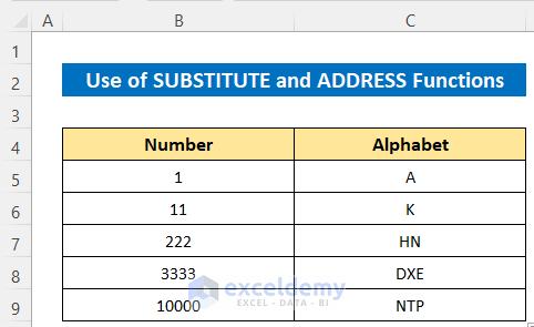
- Use the Fill Handle tool to copy the formula.
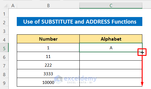
We have all the column names in the alphabet according to my given column numbers.
Formula Breakdown:
➥ ADDRESS(1,B5, 4)
The ADDRESS function will return the cell reference according to row number 1 and column number 1. So it will return as
“A1”
➥ SUBSTITUTE(ADDRESS(1,B5, 4), “1”, “”)
The SUBSTITUTE function will replace the row number with empty from the reference and will return as-
“A”
Read More: How to Title a Column in Excel
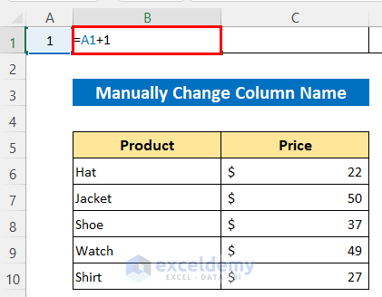
Manually Change Excel Column Name from Number to Alphabet
Steps:
- Enter 1 in cell A1.
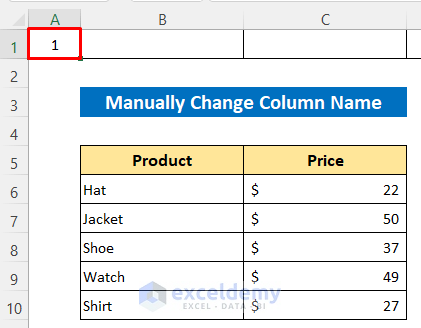
- Enter the following formula in cell B1:
=A1+1- Press the Enter button.
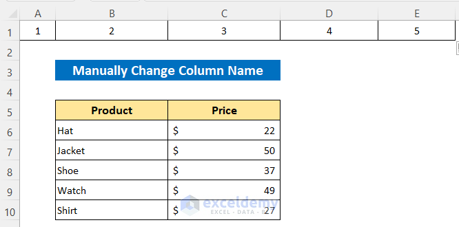
- Drag the Fill Handle icon in the right direction to get the other column numbers.
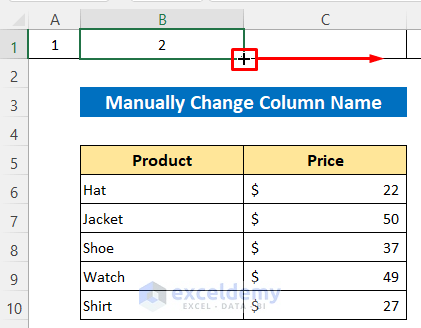
I dragged until Column E.
Read More: How to Create Excel Table with Row and Column Headers
Download the Practice Workbook
You can download the free Excel template from here and practice.
Related Articles
- How to Create Column Headers in Excel
- How to Change Column Headings in Excel
- How to Rename Column in Excel
- How to Remove Column Headers in Excel
- How to Repeat Column Headings on Each Page in Excel
- How to Remove Column1 and Column2 in Excel
<< Go Back to Rows and Columns Headings | Rows and Columns in Excel | Learn Excel
Get FREE Advanced Excel Exercises with Solutions!
