The default column name in Excel, denoted by the alphabet, does not represent the actual data that the column contains. So we need to change the column name and rename the column in Excel according to our needs. In this article, we will talk about how to rename columns in Excel.
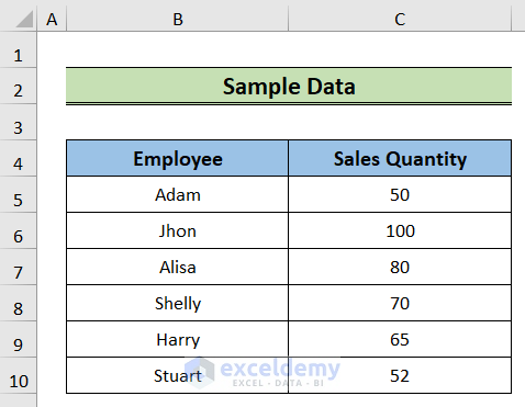
In this discussion, we will learn 3 ways to rename columns in Excel. Firstly, we will use Excel Advanced option to rename the column. Then, we will use the Formulas option to rename the column. Finally, we will use the display bar to accomplish the task. We will use the following sample dataset to illustrate the methods.
1. Using Advanced Option to Rename Column in Excel
In this method, we will hide the default column and row names and set our dataset heading as the column name. In the process, we will use the Advanced option in Excel.
Steps:
- Firstly, go to the File tab.
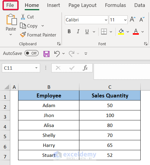
- From there, select Options.

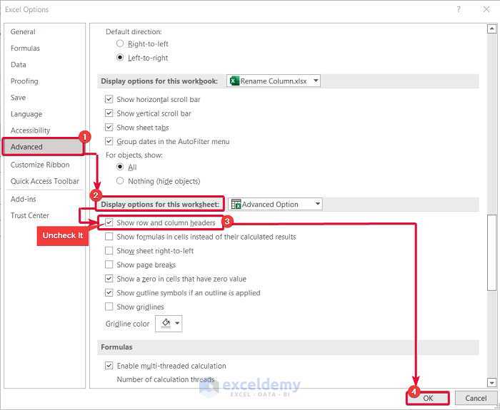
- Consequently, the Excel Options window will pop up.
- Then, select the Advanced option in the window.
- Then, hoover down to the Display options for this worksheet option.
- After that, uncheck the box beside the option Show row and column headers.
- Finally, click OK.
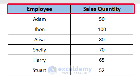
- Consequently, you will find that the dataset header is also the column name.
Read More: How to Create Column Headers in Excel
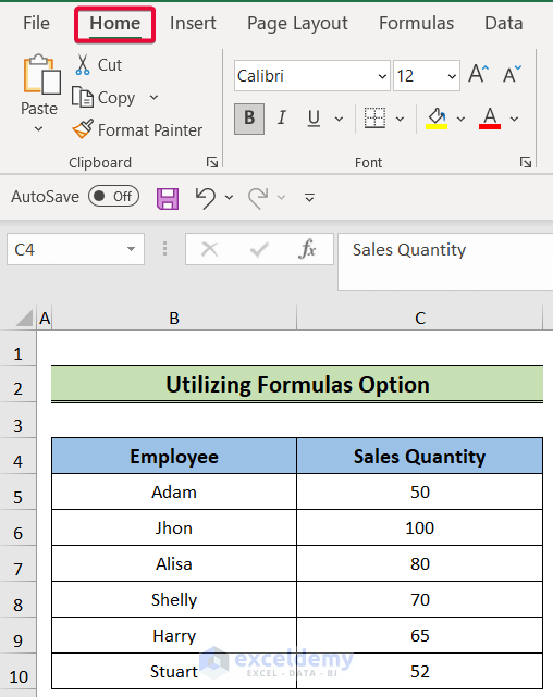
2. Applying Formulas Option to Rename Column
In this method, we will rename a column in excel with numeric values. We will use the Formulas option to do that.
Steps:
- Initially, select the File tab.
- After that, choose Options.

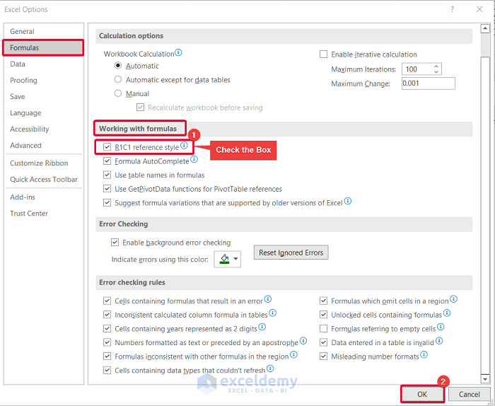
- Thus, the Excel Options window will appear.
- Then, choose Formulas.
- Following that, lower the cursor down to Working with formulas.
- You will find that the R1C1 reference style box is unchecked.

- Then, check the box.
- Finally, click OK.
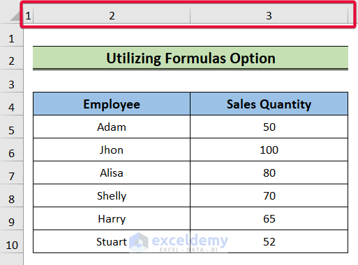
- Consequently, you will find the columns renamed in numeric format.
Read More: How to Change Excel Column Name from Number to Alphabet
3. Using Display Bar
In this final method, we will resort to the display bar to rename the columns. Follow the ensuing steps to do that.
Steps:
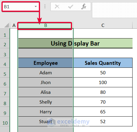
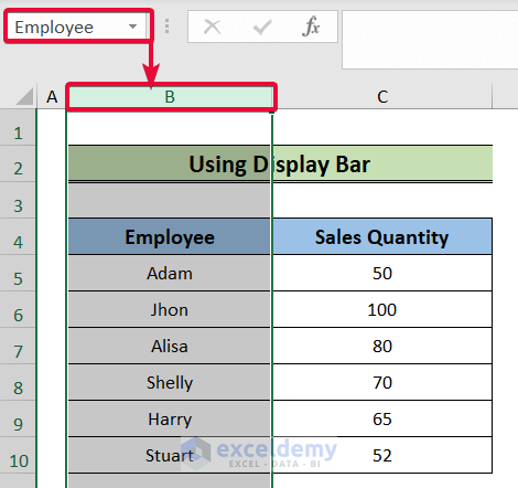
- If we click on the B column, the display bar will display B1.
- But this is ambiguous. Because we can know little about the data the column contains from that name.
- So, we will erase the name B1.

- Then, we will rename it as Employee.
- After that, we will hit Enter.
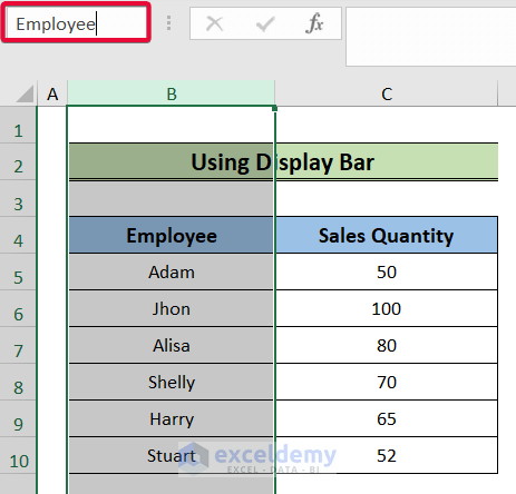
- Consequently, we will find that Excel has renamed the column from B1 to Employee.
Read More: How to Change Column Headings in Excel
How to Rename Column in Excel Power Query
In this additional method, we will rename a column using Excel Power Query. In the process, we will use the Power Query Editor.
Steps:
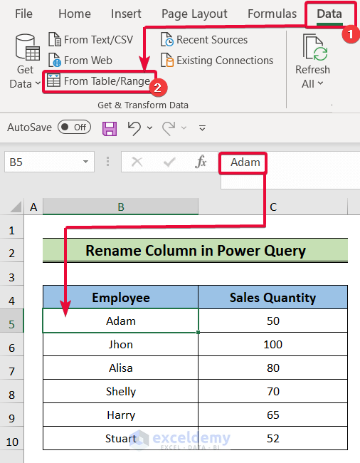
- Firstly, select any data from the dataset.
- Then, go to the Data tab in the ribbon.
- After that, select From Table/Range.
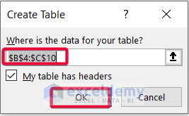
- Consequently, a prompt will appear on the screen.
- Then, in the prompt, select the dataset range as the table range.
- Finally, click OK.
- As a result, the Power Query Editor will be opened.
- In the Power Query Editor, first, go to the Transform tab.
- Then, select the Rename command.
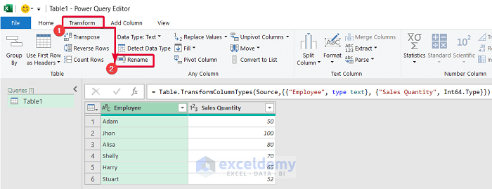
- This will take us to the column header.

- Rename the column from “Employee” to “Employee Name.”
- Then, hit Enter.
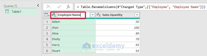
- Consequently, the column will be renamed.
- Repeat the same process for the rest of the columns.

Download Practice Workbook
Conclusion
In this article, we have talked about how to rename a column in Excel. These methods will allow users to rename the columns according to their needs and manage the data more efficiently.
Related Articles
- How to Title a Column in Excel
- How to Remove Column Headers in Excel
- How to Create Excel Table with Row and Column headers
- How to Repeat Column Headings on Each Page in Excel
- How to Remove Column1 and Column2 in Excel
- How to Change Column Header Name in Excel VBA
- [Fixed] Excel Column Numbers Instead of Letters
<< Go Back to Rows and Columns Headings | Rows and Columns in Excel | Learn Excel
Get FREE Advanced Excel Exercises with Solutions!
