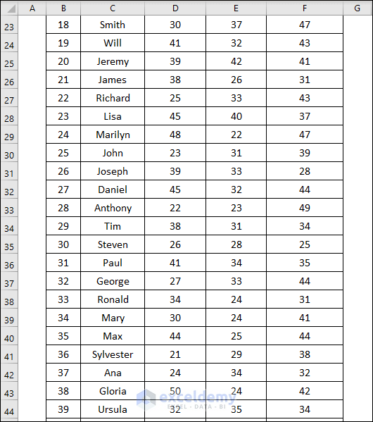
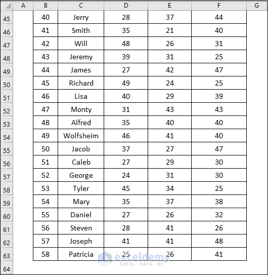
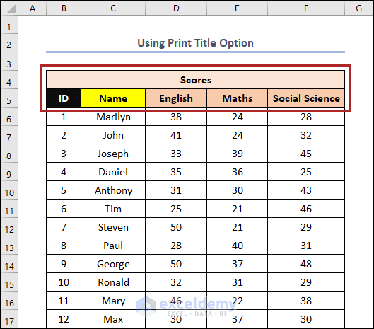
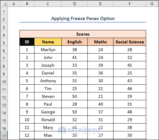
We have the Scores on the Midterm Test. Also, Row 5 includes ID, Name, English, Maths, and Social Science column headers. In the following figures, we have illustrated our dataset. We want to make Scores (Row 4) our first-row header, then make Row 5 the second row header.

Method 1 – Using the Print Title Option
Steps
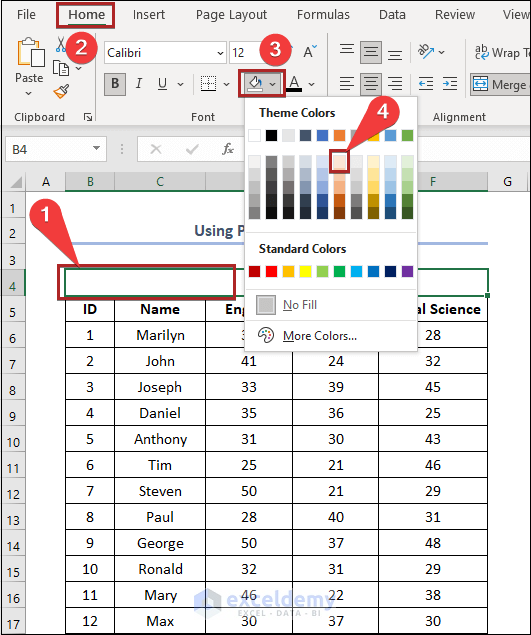
- Select cell B4.
- Go to the Home tab.
- Click the arrow next to Fill Color in the Font group.
- Choose the color Orange, Accent 2, Lighter 80%.
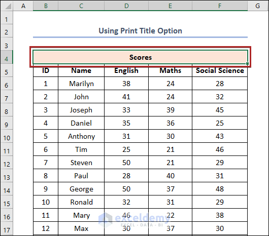
- The first-row header looks like the below one.
- Format the second-row header with colors.
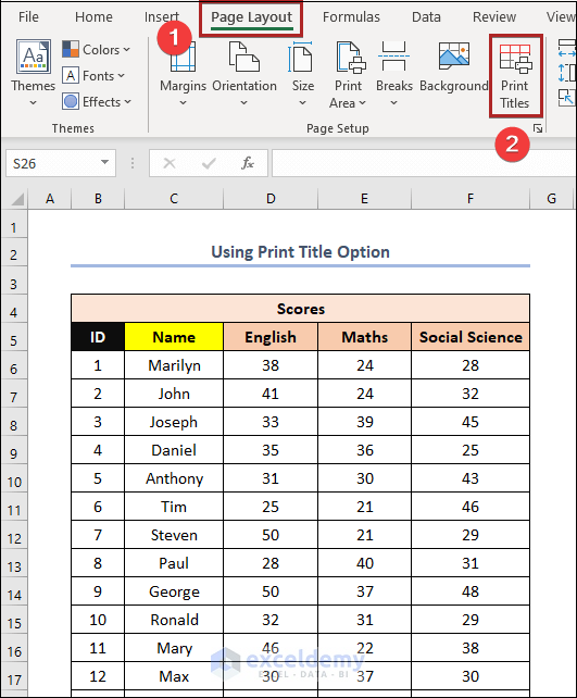
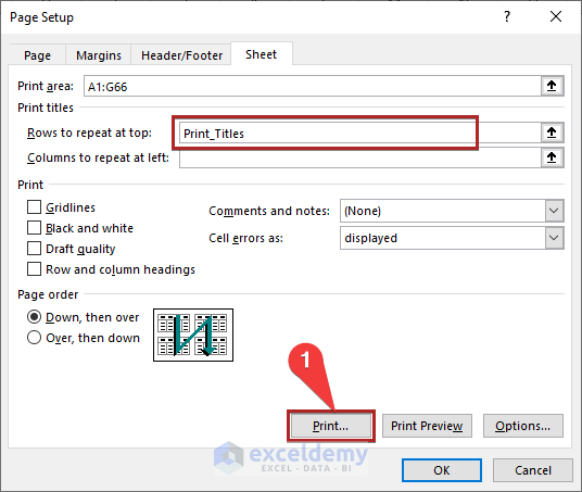
- Go to the Page Layout tab.
- Select Print Titles on the ribbon.
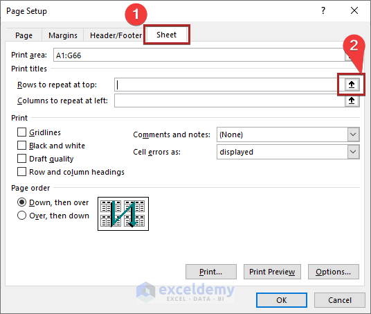
- The Page Setup dialog box opens.
- Select the Sheet tab.
- Click on the arrow in the box Rows to repeat at top.
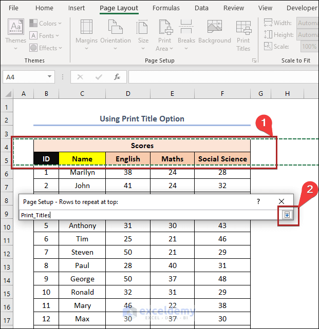
- The Page Setup dialog box becomes minimized. It opens a new wizard named Page Setup – Rows to repeat at top.
- Select Row 4 and Row 5.
- Click on the arrow in the minimized wizard.
- This returns us to the Page Setup dialog box again. We can see our selected rows in the box.
- Select the Print option.
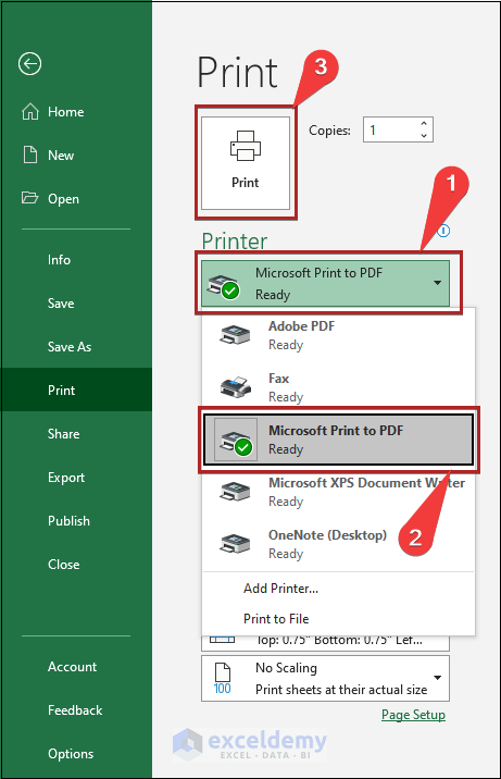
- This brings us to the Print window.
- Click on the drop-down box under the Printer option.
- Choose Microsoft Print to PDF from the available options.
- Click on the Print button.
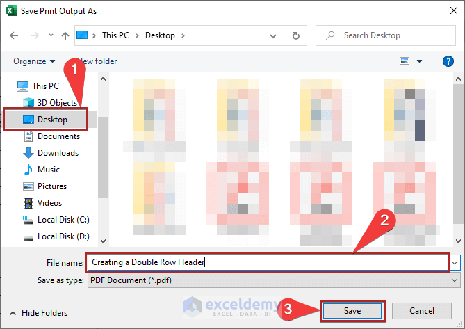
- The Save Print Output As window opens.
- Choose your desired file directory. We used Desktop.
- Write down the name of your file in the File name box.
- Click on the Save button.
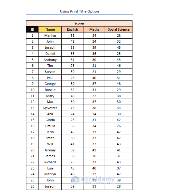
- We’ve saved our spreadsheet as a PDF.
- Open the file through a PDF reader.
- Our double-row header exists at the top of each page.

Read More: How to Make First Row as Header in Excel
Method 2 – Applying the Freeze Panes Option
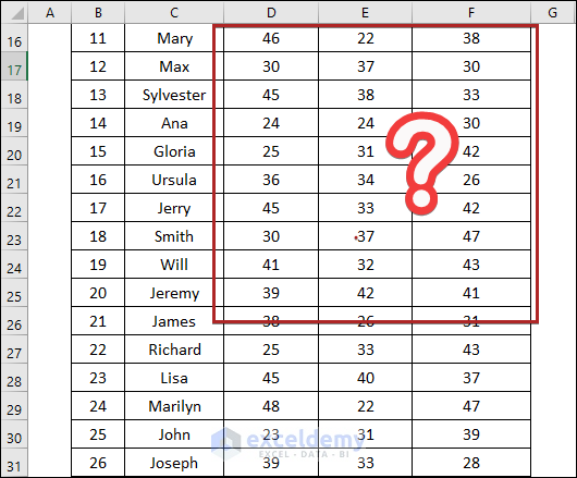
When we are at the topmost portion of our spreadsheet, we can see the header clearly.
When scrolling down, the header disappears. We’ll affix the headers to stick to the Excel pane.
Steps
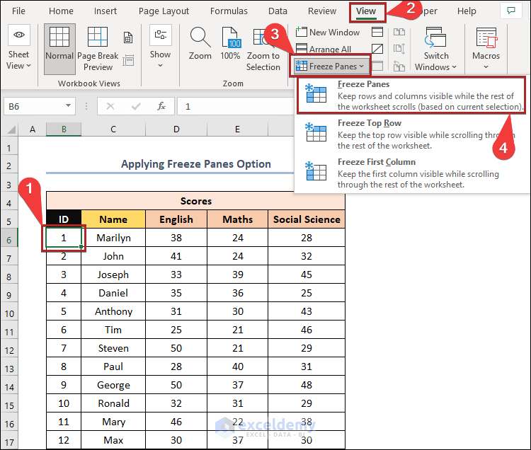
- Select cell B6.
- Move to the View tab.
- Select the Freeze Panes drop-down.
- Select the Freeze Panes option.
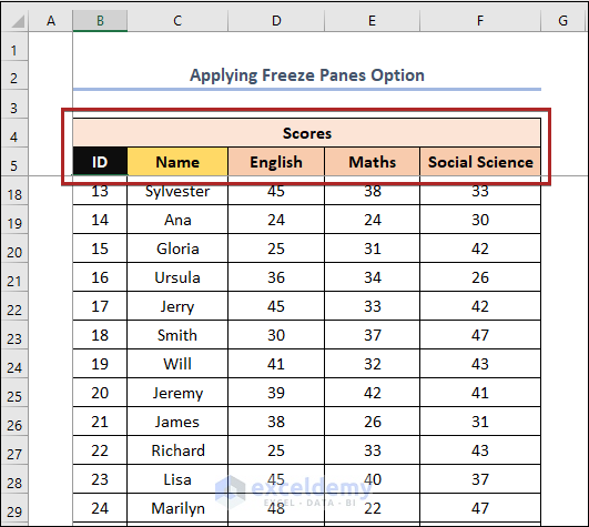
- We scrolled down to ID 13 but the Row 4 and Row 5 stayed visible.
Read More: Keep Row Headings in Excel When Scrolling Without Freeze
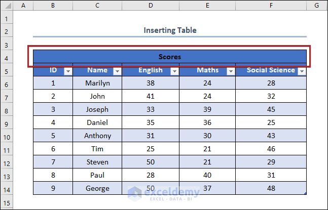
Method 3 – Inserting a Table to Create a Double Row Header
We’ve taken a portion of our dataset. We’ve shown the Scores of three subjects of the individuals with IDs 1 to 9.

Steps
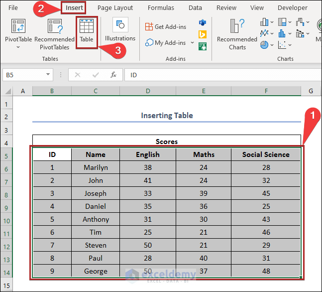
- Select the cells in the B5:F14 range.
- Go to the Insert tab.
- Select Table from the Tables group.
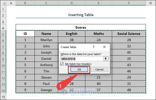
- A Create Table input box opens.
- We can see our selected range of cells present in the Where is the data for your table? box.
- Check the box of My table has headers.
- Click OK.
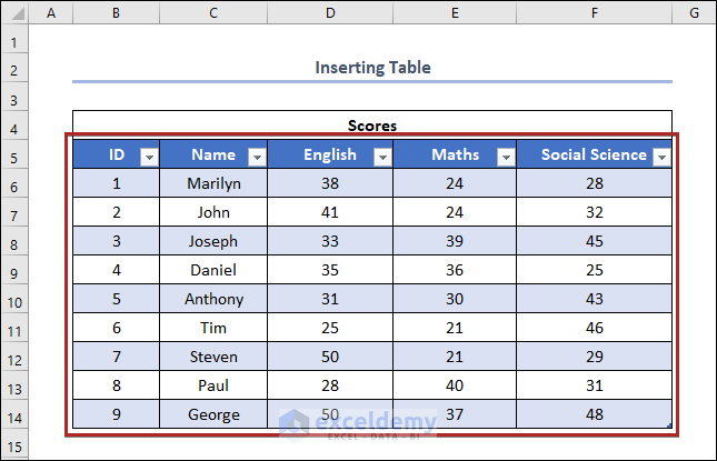
- We converted the selected range into a Table.
- The headers have the Filter Buttons.
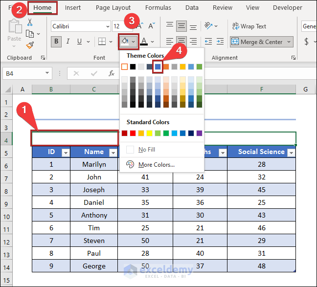
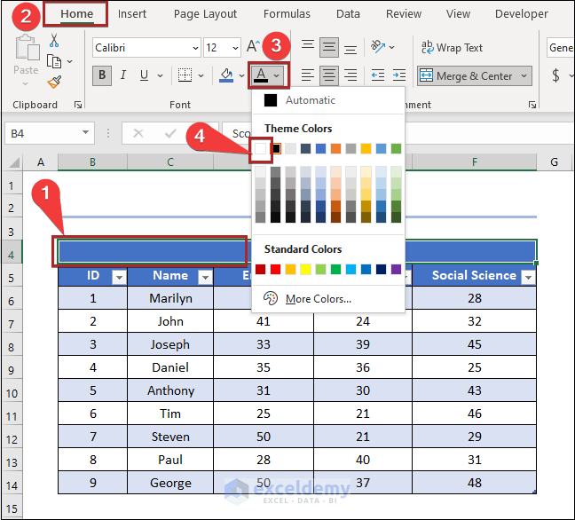
- Select cell B4.
- Go to the Home tab.
- Click the arrow next to Fill Color in the Font group.
- Choose the color Blue, Accent 1.
- Here’s the format.
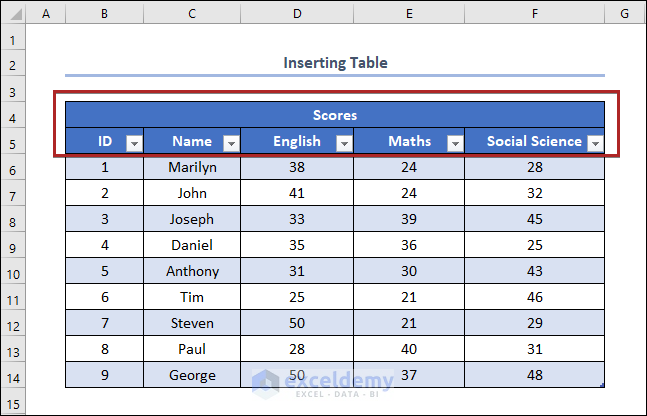
- Select cell B4.
- Go to the Home tab.
- Click the arrow next to Font Color in the Font group.
- Choose the color White, Background 1.
- Our Table looks like it has a double-row header.
Read More: How to Make a Row Header in Excel
Download the Practice Files
Related Articles
<< Go Back to Rows and Columns Headings | Rows and Columns in Excel | Learn Excel
Get FREE Advanced Excel Exercises with Solutions!
