When using Microsoft Excel, sometimes we need to hide row and column headings to represent our dataset. This is a very basic Excel operation. Are you having trouble hiding the row and column headings in Excel? This article will help to learn how to hide row and column headings in Excel in 2 suitable ways. Let’s get started!
How to Hide Row and Column Headings in Excel: 2 Suitable Ways
There are 2 ways to hide row and column headings in Excel. One of them is using the View tab and another one is using the Excel Options window. Both ways are very easy and efficient to do the task. Now we will learn how to hide row and column headings in these 2 ways.
1. Use of View Tab to Hide Row and Column Headings in Excel
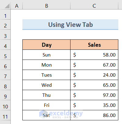
This method is quicker and easier than the second method. Suppose, you have a dataset like the following figure and you want to hide row and column headings for the dataset. In order to hide row and column headings by using the View tab, follow the steps below.
Steps:
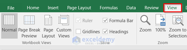
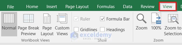
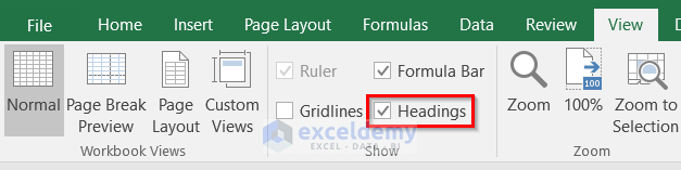
- First of all, click on the View tab from your ribbon.
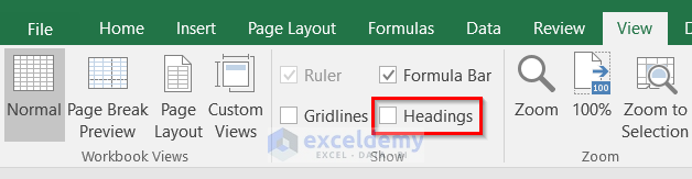
- After that, uncheck the Headings option like the image below.
- As a result, you will see that your row and column headings are hidden from your worksheet as shown below.

Read More: How to Make a Row Header in Excel
2. Hide Row and Column Headings from Excel Options Window
We can also hide row and column headings from the Excel Options window. This method is also an easy and efficient one to do the task. Suppose, we have a dataset like the image below and we want to hide the headings from the Excel Options window. Follow the steps below to hide the headings from the Excel Options Window.
Steps:
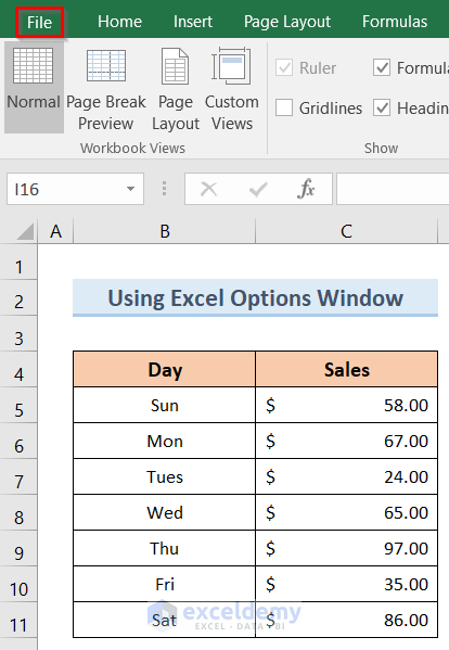
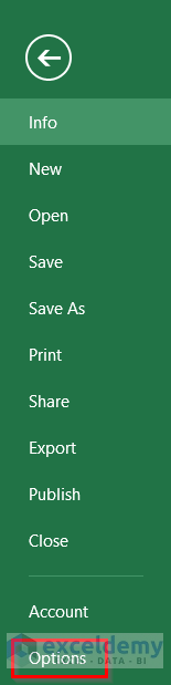
- First, click on the File Tab from your ribbon as shown below.
- Then, click on the Options like the image below.
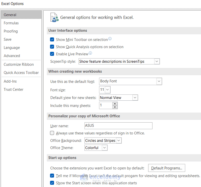
- As a result, Excel Options window will pop up on your screen like the below one.
- After that, click on the Advanced option and scroll down your screen until you find the Display option for this worksheet menu like the following image.
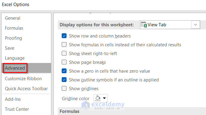
- Furthermore, uncheck the Show row and column header option as shown below.

- Hence, click OK.

- As a result, you will now see that your row and column headings are hidden from your worksheet like the image below.

Read More: How to Make First Row as Header in Excel
How to Unhide Row and Column Headings in Excel
After hiding row and column headings, if we want to unhide the headings in Excel, we can do it like the above-described methods as well. Suppose, we have a dataset like the following figure and we want to unhide the row and column headings for the dataset. In order to unhide row and column headings, we have to follow the steps below.

Steps:
- To start with, click on the View tab from your ribbon.
- After that, check the Headings option like the image below.
- As a result, you will see that your row and column headings are unhidden from your worksheet like the image below.

Read More: How to Create a Double Row Header in Excel
Things to Remember
- First of all, If you want to be really quick and efficient in using Excel, then Using the View tab method will be the best option for you to hide the headings.
- Moreover, you can also unhide row and column headings using the above-described 2 methods.
Download Practice Workbook
You can download the Excel workbook from here.
Conclusion
Hence, follow the above-described methods. Thus, you can quickly learn how to hide row and column headings. Hope this will be helpful. Don’t forget to drop your comments, suggestions, or queries in the comment section below.
Related Articles
- How to Make Multiple Sortable Headings in Excel
- Keep Row Headings in Excel When Scrolling Without Freeze
- How to Keep Row Headings in Excel When Scrolling
- How to Promote a Row to a Column in Excel
<< Go Back to Rows and Columns Headings | Rows and Columns in Excel | Learn Excel
Get FREE Advanced Excel Exercises with Solutions!
