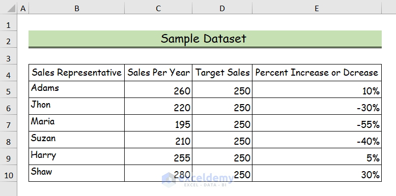
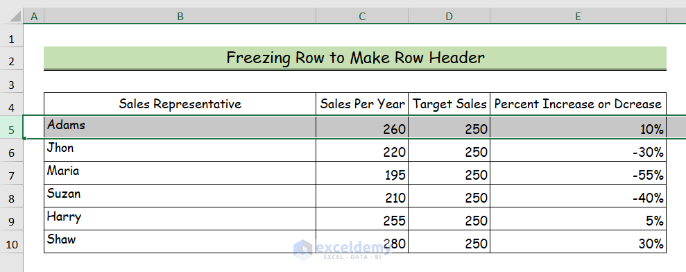
Here, we have provided a sample dataset that we will use to make a header row in Excel. As you can see, it’s not particularly distinct from the data.
Method 1 – Customizing Formats to Make a Row Header in Excel
Steps
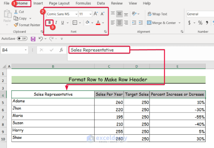
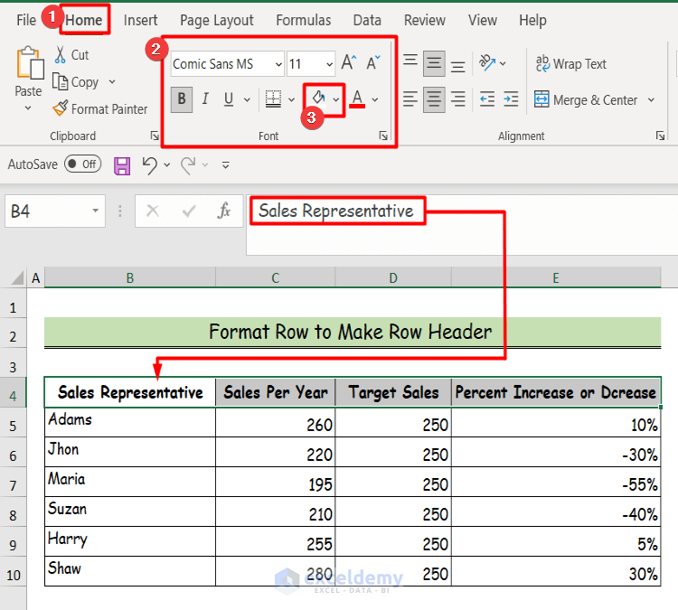
- Select the columns from the row that you want to make a row header. We will select the cells B4:E4.
- Go to the Home tab in the ribbon.
- Go to the Font group.
- Click on the capital B, which stands for Bold Text.
- The text in the selected cell will become bold.
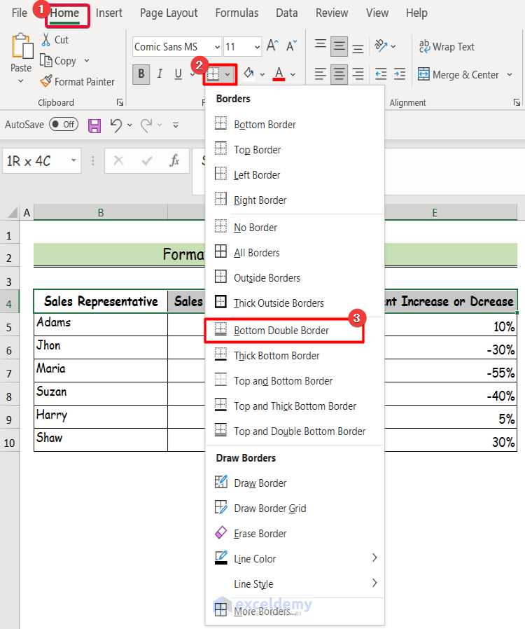
- Keep the cells selected.
- Select the Border tool in the Font group.
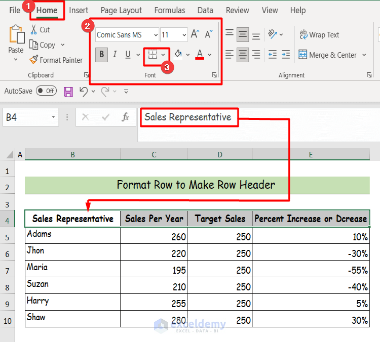
- From the drop-down list, select any border. Here, we have chosen the Bottom Double Borderoption.
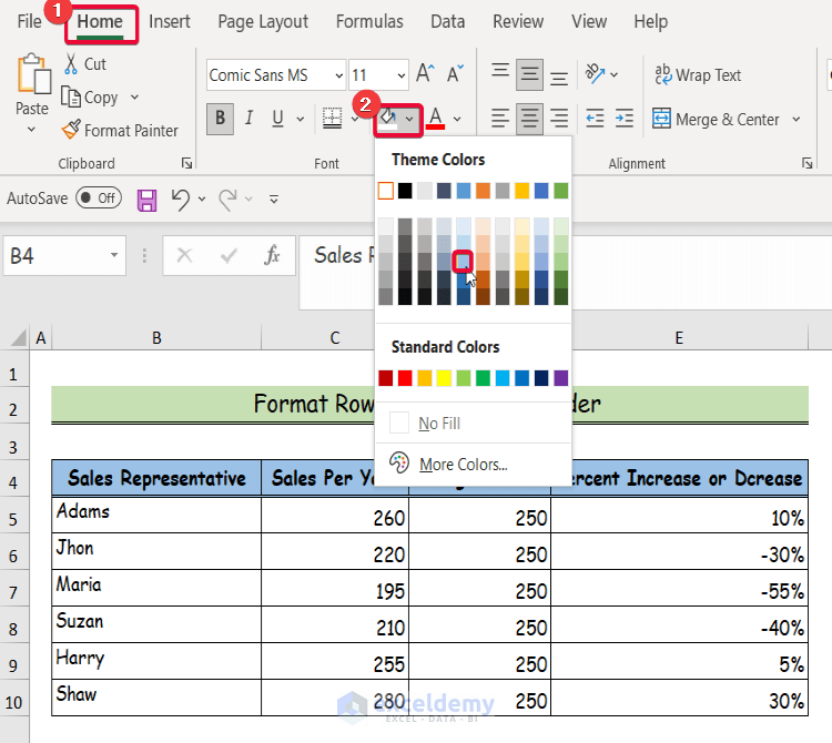
- Click on the icon next to the Border. This is the Fill Color tool.
- From the drop-down list of the Fill Color tool, choose any of your preferred colors. In this instance, we chose a shade of blue.
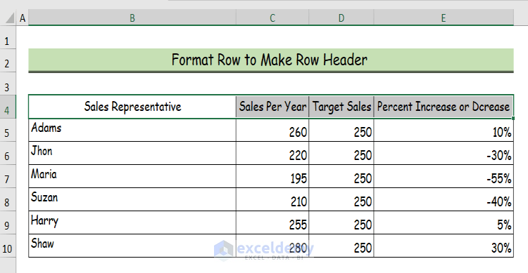
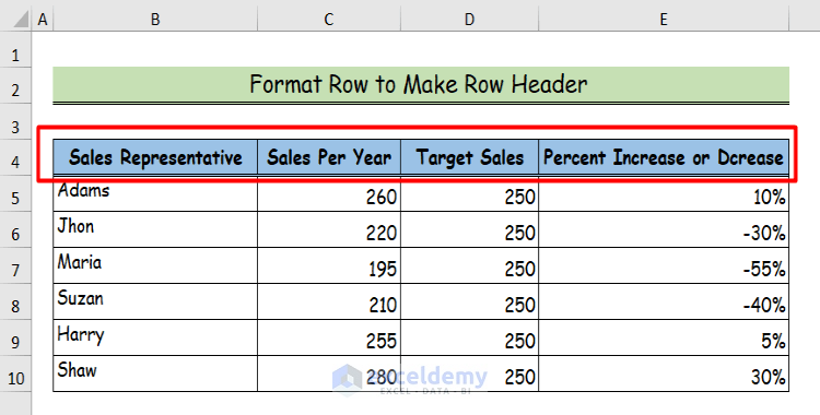
- This is our vivid row header.
Read More: How to Make First Row as Header in Excel
Method 2 – Freezing Row to Make a Row Header in Excel
Steps:
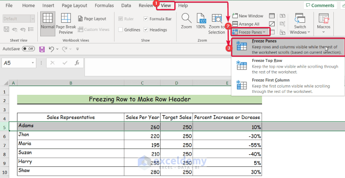
- Select a row just after the desired row that you want to turn into a header row. In this case, we selected Row 5.
- Go to the View tab in the ribbon.
- Select the Freeze Panes tool.
- From the drop-down list, select the Freeze Panes command.
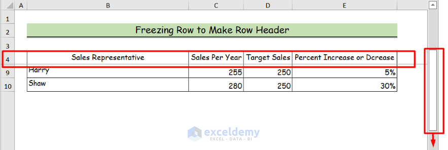
- As you scroll, the other rows will move up and down except for Row 4.
Read More: How to Hide Row and Column Heading in Excel
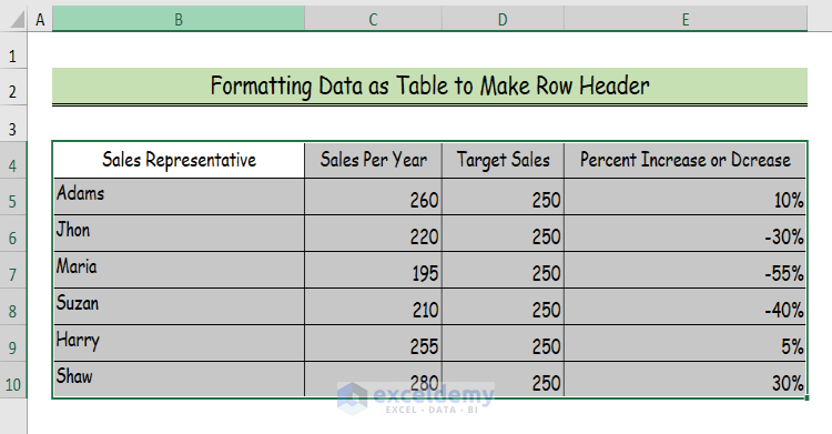
Method 3 – Formatting Data as Excel Table to Make a Row Header
Steps:
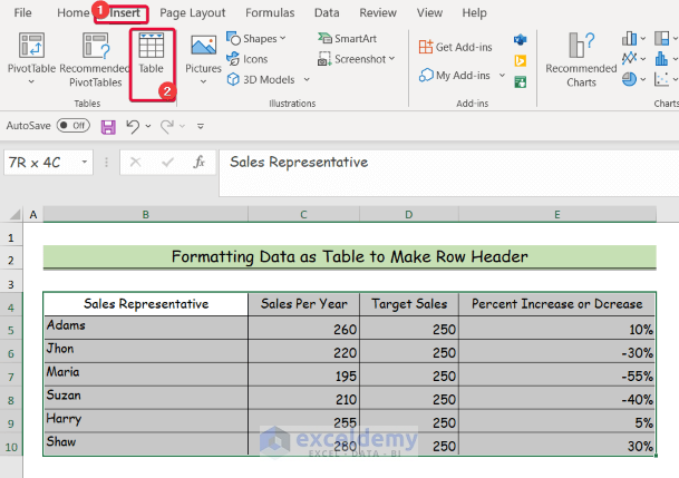
- Select the cells containing the entire data set. We selected the cells in B4:E10.
- Go to the Insert tab in the ribbon.
- Click on the Table tab.
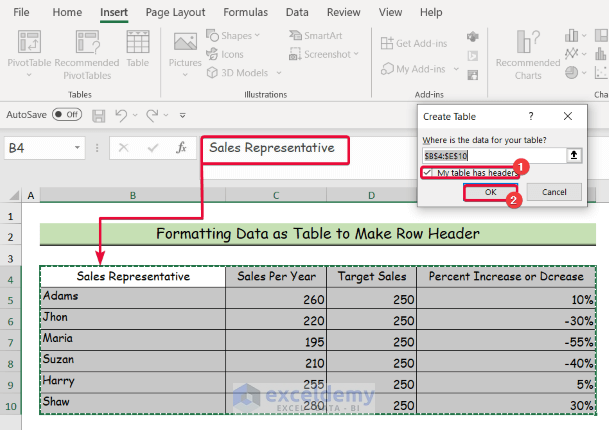
- A Create Table dialogue box will appear.
- Check the checkbox that contains the text “My table has headers.“
- Click OK.
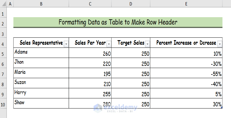
- There is now a row header at the top of the table.
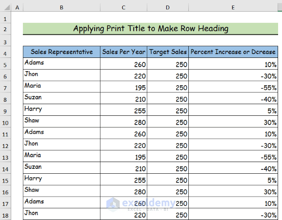
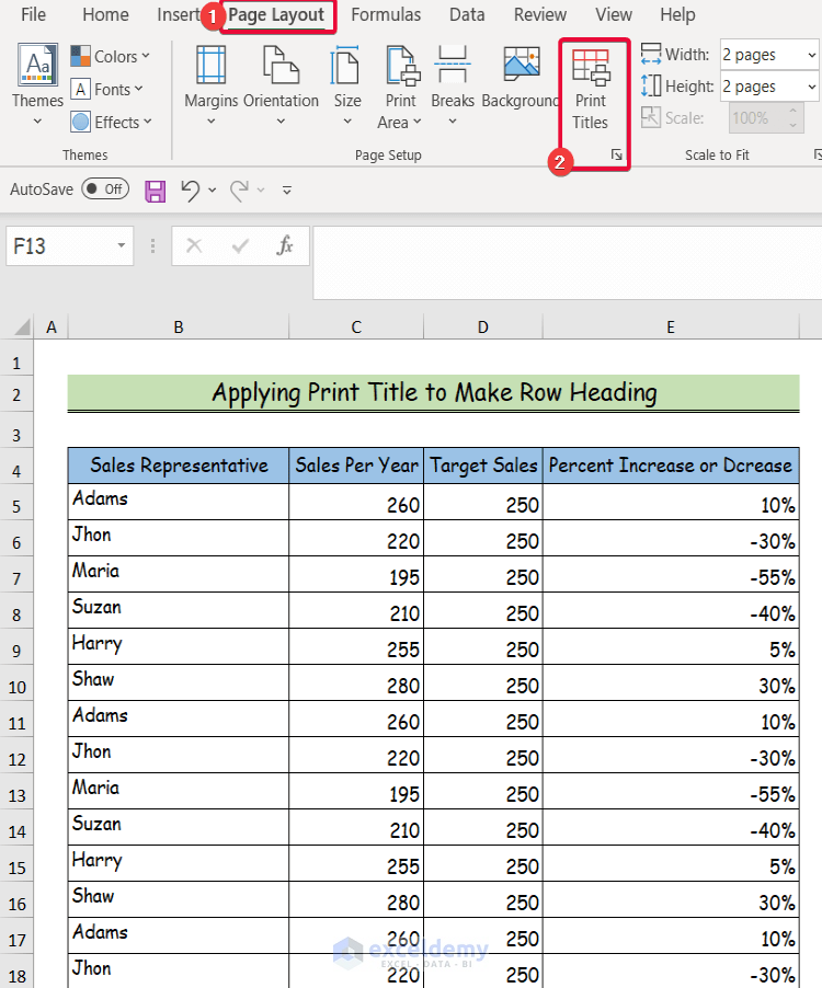
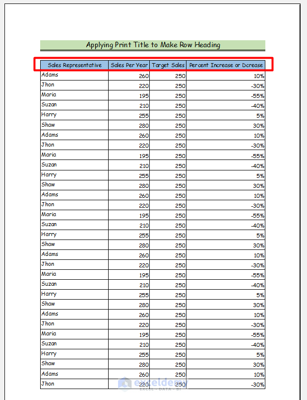
Method 4 – Inserting Print Title to Make a Row Header in Excel
Here, we have a dataset that will exceed one page when we print it out. We will ensure each printed page has the same header row.
Steps:
- Go to the Page Layout tab.
- Select the Print Title command.
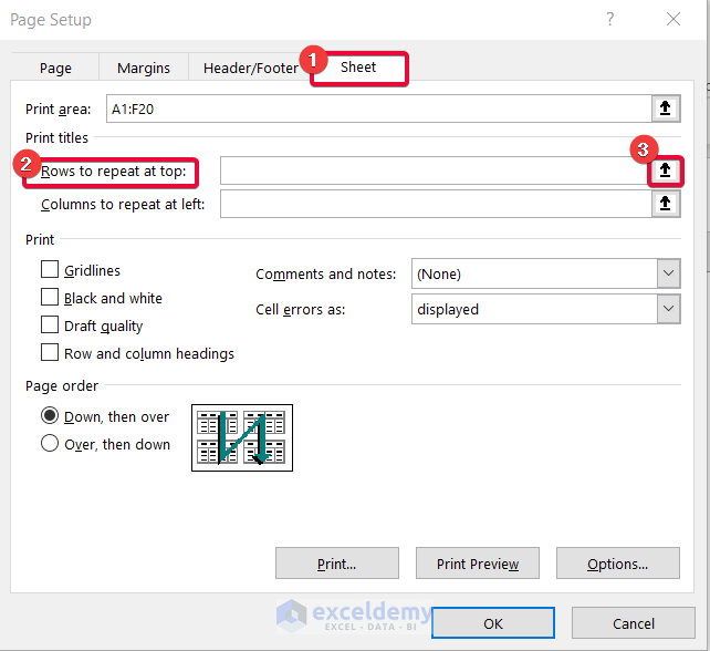
- The Page Setup dialogue box will appear.
- Select the Sheet tab.
- Go to Rows to repeat at the top command box.
- Click on the upward arrow at the right-hand side.
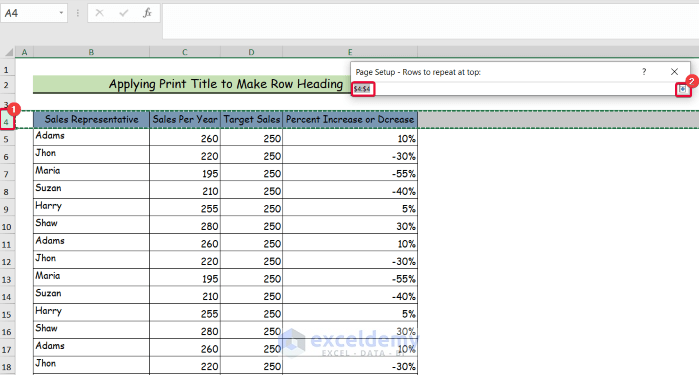
- Select the desired row that you want as a row header. In this instance, we will select row 4, marked as $4:$4 in the command box.
- Click on the upward arrow to the right of the command box to confirm selection.
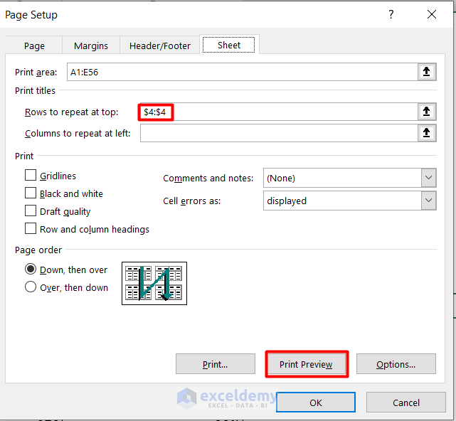
- In the Page Setup dialogue box, the selected row will appear in Rows to repeat at the top command box.
- Click on the Print Preview tab.
- You will have a preview of the first page that will be printed.
- If you slide down, you will see the second page. The page contains the same row header as the first page.
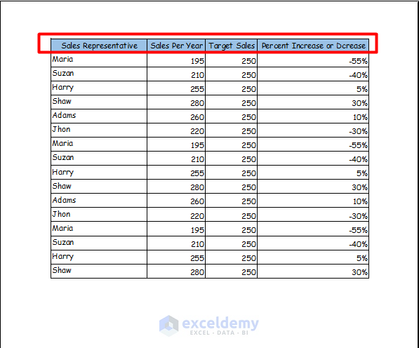
Note: While checking for print preview make sure to check the Page Break option. This will ensure that the data is printed properly on all the pages.
Read More: How to Create a Double Row Header in Excel
Download Practice Workbook
You may download the following Excel workbook for better understanding and practice yourself.
Related Article
<< Go Back to Rows and Columns Headings | Rows and Columns in Excel | Learn Excel
Get FREE Advanced Excel Exercises with Solutions!
