How to Transpose Column to Multiple Rows in Excel: 6 Methods

Method 1 – Using Excel TRANSPOSE Function to Transpose Column to Multiple Rows

Steps:

Type the following formula in cell B12.

=TRANSPOSE(B4:D10)

The TRANSPOSE Function returns the transpose of the array B4:D10, meaning it will convert the columns and rows of B4:D10 to rows and columns.

Press ENTER, and you will see this operation transpose the whole dataset.

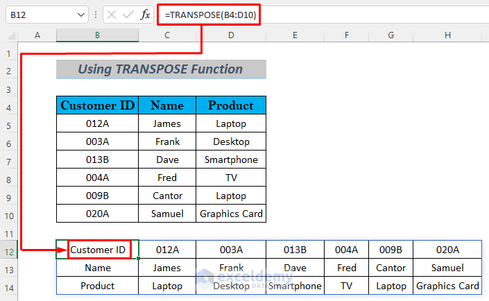
You can easily transpose columns to multiple rows simply by using the TRANSPOSE Function.

Method 2 – Applying Combination of Functions to Transpose Column to Multiple Rows in Excel

Steps:

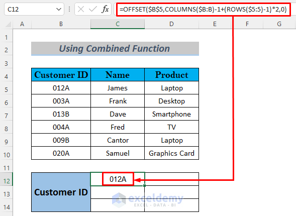
Make a heading for Customer ID and type the following formula in cell C12.

=OFFSET($B$5,COLUMNS($B:B)-1+(ROWS($5:5)-1)*2,0)

Formula Breakdown

We used the OFFSET Function to return values taking the B5 cell as a reference. It will return a range with a particular number of columns and rows from reference B5.

ROWS($5:5)-1 —-> Returns
- Output: 0
(ROWS($5:5)-1)*2 —-> Returns (We multiply this formula by 2 because the return array will be a 3×2 Matrix, and we want 2 cells in each row)
- Output: 0
COLUMNS($B:B)-1 —-> Becomes
- Output: 0
COLUMNS($B:B)-1+(ROWS($5:5)-1)*2 —-> Turns into
- Output: 0
OFFSET($B$5,COLUMNS($B:B)-1+(ROWS($5:5)-1)*2,0) —-> Simplifies to
OFFSET($B$5,0,0) —-> The OFFSET function offsets B5 Offsets 0 row and 0 column and will return the value of the B5 cell.
- Output: “012A”

We get the cell value of B5.

Hit ENTER and you will see the first Customer ID in this cell.

Now use the Fill Handle to AutoFill the adjacent cell D12.

Drag the Fill Handle icon vertically to cell D14 and you will see the Customer IDs in a 3×2 Matrix

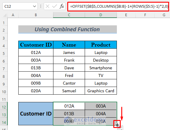
You can transpose a single column into multiple rows by combining OFFSET, ROWS, and COLUMN Functions.

Method 3 – Implementing Excel INDEX Function to Transpose Column to Multiple Rows

Steps:

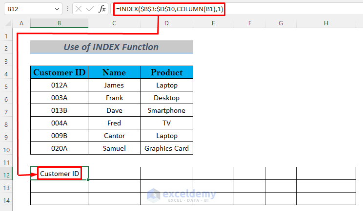
Type the following formula in cell B12.

=INDEX($B$3:$D$10,COLUMN(B1),1)

We define the COLUMN Function as the row_number for the INDEX Function as we want to make the columns as rows. The COLUMN(B1) formula will return the Column number of that cell reference which is 2 (You may use any cell reference from Column B). Then INDEX looks in the range $B$3:$D$10 and returns the value which is in the 2nd row and 1st column of the range $B$3:$D$10. In this case, the output value will be Customer ID.

Hit ENTER and you will see the Customer ID header appear in cell B12.

The following formula similarly in cell B13 and hit ENTER to see the Name

=INDEX($B$3:$D$10,COLUMN(B1),2)

Type the following formula in cell B14 and press ENTER to see the Product header similarly.

=INDEX($B$3:$D$10,COLUMN(B1),3)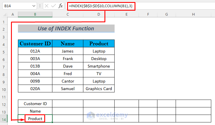

Select B12:B14 and drag the Fill Handle icon horizontally to H14. The whole dataset will become transposed.

You can transpose columns to multiple rows by using INDEX and COLUMN Functions.

Method 4 – Transposing Column to Multiple Rows by Excel INDIRECT Function

Steps:

Type the following formula in cell B12.

=INDIRECT("B"&COLUMN(D5))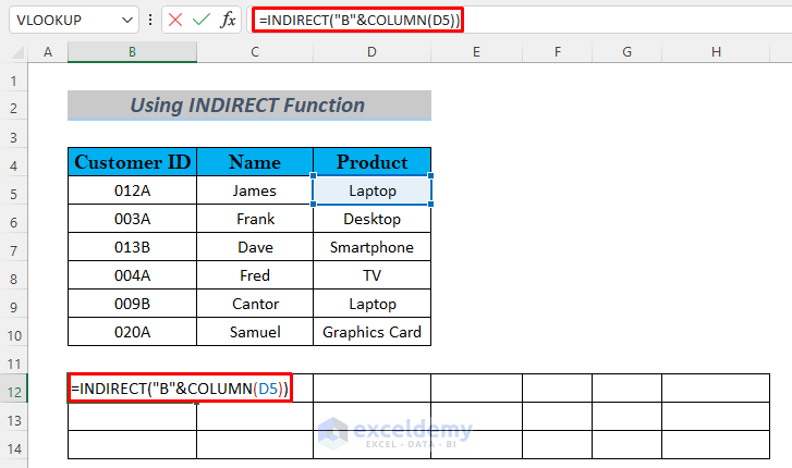

We want to make Columns B, C, and D of the dataset as rows. We put a reference in the INDIRECT Function. The COLUMN(D5) formula will return the column number of this cell reference which is 4. Our dataset also starts at the 4th row. Use any of the cell references from column D for the COLUMN Function. We get the cell value of B4, which is Customer ID.

Hit ENTER and you will see the Customer ID header appear in cell B12.

Type the following formula similarly in cell B13 and hit ENTER to see the Name

=INDIRECT("C"&COLUMN(D5))

Type the following formula in cell B14 and press ENTER to see the Product header similarly.

=INDIRECT("D"&COLUMN(D5))

Select B12:B14 and drag the Fill Handle icon horizontally to H14. The whole dataset will become transposed.

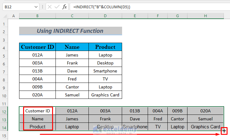
Thus you can transpose columns to multiple rows by using INDIRECT and COLUMN Functions.

Method 5 – Utilizing Cell Reference to Transpose Column to Multiple Rows

Steps:

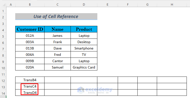
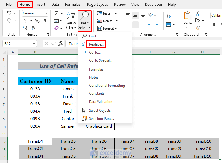
Select any empty cell from where you want to transpose your dataset. I selected B12 and typed TransB4 instead of the formula ‘=B4’. Trans is a homemade prefix.

Type TransC4 and TransD4 in cells B13 and B14

Select B12:B14 and drag the Fill Handle icon horizontally up to H14.

Go to Home >> Find & Select >> Replace.

A dialog box will show up. You want cell values in the transposed So you need to replace ‘Trans’ with the EQUAL symbol (‘=’). So type Trans in Find what section and ‘=’ in Replace with section.
Click Replace All.

A message box will show up showing how many changes this operation made. Click OK.

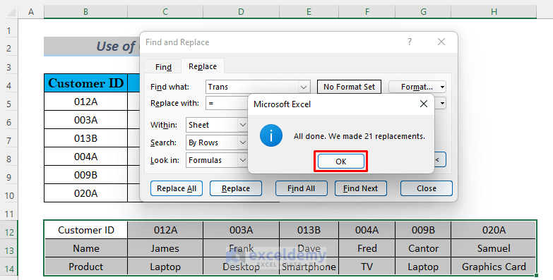
Close the Find and Replace dialog box.

You can transpose columns to multiple rows by using cell reference.

Method 6 – Using VBA to Transpose Column to Multiple Rows

Steps:

Open Visual Basic from the Developer Tab.

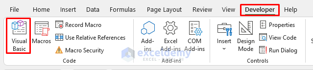
The VBA Window will open. Select Insert >> Module.

Type the following code in the VBA Module.

Sub TransposeToColumn()
steps = 2
FR = 5
FC = 2
New_FC = 3
New_FR = 12
New_Current_Column = New_FC
New_Current_Row = New_FR
LR = Cells(Rows.Count, FC).End(xlUp).Row
For CR = FR To LR
    Cells(New_Current_Row, New_Current_Column).Value = Cells(CR, FC).Value
    New_Current_Column = New_Current_Column + 1
    If (CR - (FR - 1)) Mod steps = 0 Then
        New_Current_Column = New_FC
        New_Current_Row = New_Current_Row + 1
    End If
Next
End Sub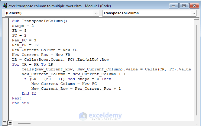

Code Breakdown

Define steps equal to 2 as we want 2 cells in each row.
Our first value is in cell B5 so we define First Row (FR) as 5 and First Column (FC) as 2.
We will store the values in cell C12 so we define New First Column (New_FC) as 3 and New First Row (New_FR) as 12.
We also define Last Row (LR) to keep the last used row number.
We used a For Loop to go through from FR row 5 to LR, row 10.
The values of the previous cell in the new New_Current_Row and New_Current_Column. Increment the New_Current_Column value by 1.
The VBA Mod operator was used within the IF statement to transpose the rest of the values. Also incremented New_Current_Row by 1.