Many times in Excel, we do not get the required data in the appropriate orientation. Sometimes we may need to flip the columns and rows to make the data more convenient to read. In this article, we will see how to flip columns and rows in Excel.
How to Flip Columns and Rows in Excel: 2 Simple Methods
In this section, we will demonstrate 2 easy and effective ways to flip Columns and Rows. Let’s start.
1. Apply Paste Special Method to Flip Columns and Rows
Paste Special is perhaps the most convenient way to flip/transpose rows into columns or vice versa. We will step by step explore how the method works.
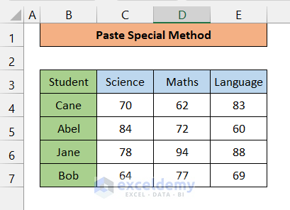
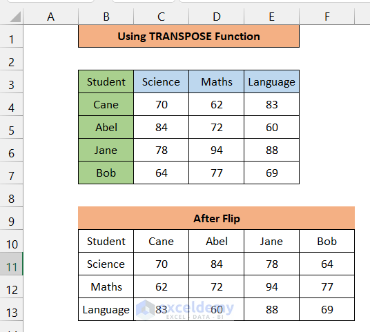
To illustrate the method, we have chosen an example in which an array is given containing marks of 3 subjects for 4 students. The subjects are distributed in columns and students are distributed in rows. But now we want to represent the data in a different way. The students will be in columns and the subjects will be in the row.
Follow the steps mentioned below to perform this flip.
Step 01:
- Select the entire cells you want to flip. Here we have selected from B3 to E7.

Step 02:
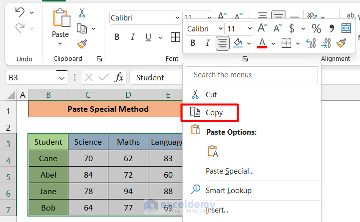
- Type Ctrl+C to copy or right-click on the mouse and select copy option.
Step 03:
- Choose the topmost left cell in the location in which you want to relocate your flipped data. Here we have chosen cell B10.

Step: 04:
- Right-click on the mouse and you will see a window popped up containing Paste Options.
- Under this, you will see many types of paste functions. Among those, you need to click on the Transpose (marked by a red box in the picture below)

You can also access Paste Special Options by typing CTRL+ALT+V. A window will pop up like this.
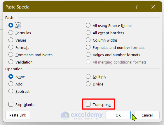
And now you have to check the Transpose and click OK.
- The columns and rows will get interchanged. The result will be as below:

Note:
- Here we can see that we also duplicated the cell color and font color.
- The flipped array and the first array are not directly linked. For instance, you can change any value in the first array, but the corresponding value in the flipped array will remain unchanged.

Read More: How to Transpose Multiple Columns to Rows in Excel
2. Use TRANSPOSE Function to Flip Columns and Rows
The TRANSPOSE function is also an effective way to flip columns and rows in Excel. Scroll down to see the steps:
Step 01:
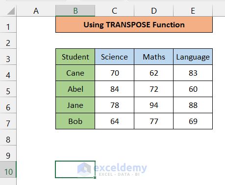
- At first, select the top most cell in which you want to relocate your swapped array. Here we have selected B10.
Step 02:
- Now type “=TRANSPOSE” and you will see a function popping up like below.
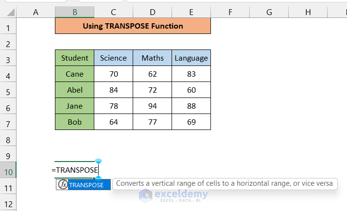
- Now, click on the popup. Now you have to select the array you want to work with. Here, we have selected B3:E7.
- So, the Function is,
=TRANSPOSE(B3:E7)
Step 03:
Now click Enter. You will see the following result.
Note:
- Beware that we did not maintain cell format in this method. Therefore, we can see that we have not copied the cell color. But the font color will be the same.
- The flipped array is directly linked to the first array. As a result, if we change any value in the first array, the exact change will occur in the flipped array as well.
- We can not change the value of the flipped array. If we try to input any data manually in the flipped array, an error will be shown like this.
Read More: How to Flip Data from Horizontal to Vertical in Excel
Download Practice Workbook
Download the following workbook to practice by yourself.
Conclusion
When it comes to representing data from a different perspective, flipping rows and columns is a very handy tool. Knowing how to flip columns and rows will give you the power to easily and quickly check the representation of your data in an alternate way.
Related Articles
- How to Convert Multiple Rows to Columns in Excel
- How to Paste Link and Transpose in Excel
- How to Move Data from Row to Column in Excel
- How to Change Vertical Column to Horizontal in Excel
- Excel VBA to Transpose Array
- Excel Macro: Convert Multiple Rows to Columns
- VBA to Transpose Multiple Columns into Rows in Excel
<< Go Back to Transpose Data in Excel | Learn Excel
Get FREE Advanced Excel Exercises with Solutions!
