Convert Columns to Rows in Excel Using Power Query

In this tutorial, we will describe how to convert columns to rows in Excel using Power Query.

What is Power Query in Microsoft Excel?

Power Query, also known as “Get & Transform Data“, is a powerful tool used to clean and automate data. The uses of Power Query can be divided into two main categories:

Get Data: Import data into Excel from sources such as databases, csv files, other Excel files, or web pages.

Transform Data: Imported data can then be cleaned and arranged, for example adding or merging columns.

Power Query is only available on Windows PCs, and from Excel 2010 onwards. For Excel 2010 or Excel 2013, download Power Query from the Microsoft website and install it as an Excel Add-in. From Excel 2016 onwards, Power Query is pre-installed as a built-in feature.

Format the Data as a Table to Convert Columns to Rows Using Power Query

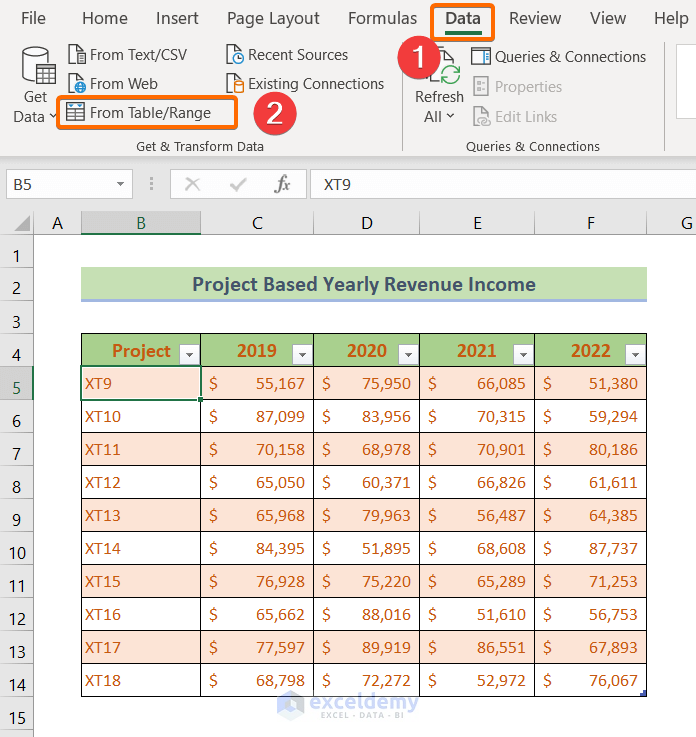
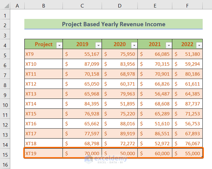
We’ll use the following dataset to demonstrate the conversion process from columns to rows using Power Query.

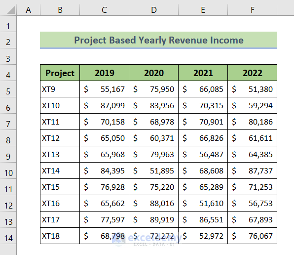
Before we can apply Power Query, we’ll have to convert this dataset into an Excel table.

Steps:

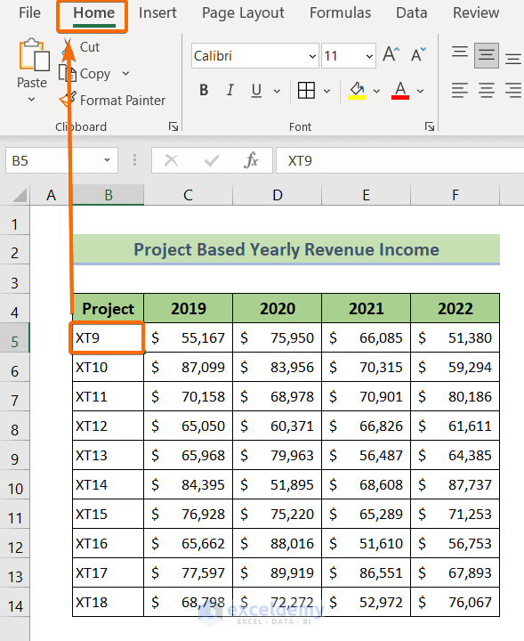
Click on a cell of the dataset.
Go to the Home tab on the main ribbon.

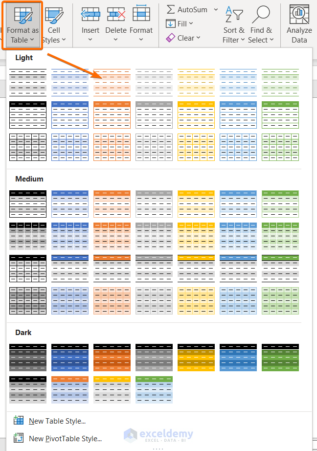
Click on the Format as Table drop-down.
Select a table format from the options.

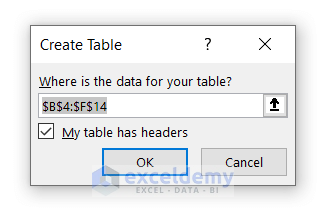
The Create Table dialog box will appear with the selected cell range pre-loaded.

Click OK to create an Excel Table.

Read More: How to Transpose a Table in Excel

Use Power Query to Convert Columns to Rows

We are now ready to apply the Power Query.

Steps:

Click on any cell of the data table to select it.
Go to the Data tab.
Under the Get & Transform data group, click on From Table/Range.

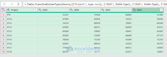
A new window called Power Query Editor will appear.

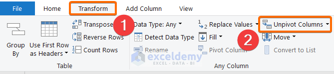
Select the columns to convert to rows.

Go to the Transform tab.
From the Any Column group, click on Unpivot Columns.

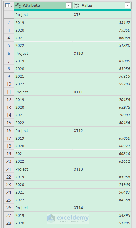
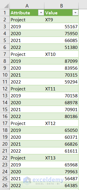
The specified columns are converted to rows, as in the picture below:

Live Update of the Data in the Excel Table

Transposing using the Power Query enables us to instantly insert and update data in Excel data tables.

Steps:

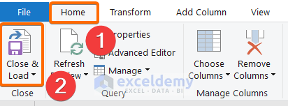
Go back to the Home tab of the Power Query Editor.
From the Close group, choose Close & Load.

Excel will create a new worksheet to display the converted version of the raw table, where the columns have been converted into rows.

Update the original data table, for example like here in row 15.

Right-click anywhere on the Excel table just created using the Power Query.
From the pop-up list, choose Refresh.

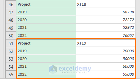
After refreshing the worksheet, the data table is updated. The newly added data have already been converted from columns to rows, as in the screenshot below: