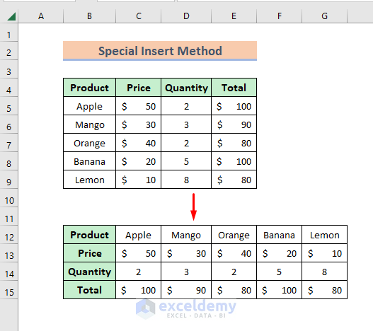
Method 1 – Using Paste Special Tool to Transpose a Table in Excel
STEPS:
- Select the whole table using a mouse.
- Press Ctrl + C, and a dancing rectangle will appear at the border of the selected range of cells.
![]()
- Activate a new cell where you will transpose the table. We activated cell B12.
- Press Ctrl + Alt + V, and the Paste Special box will pop up.
- Mark the Transpose box and press OK.
![]()
- See the table has been transposed to the new location.
Method 2 – Inserting TRANSPOSE Function to Switch a Table
STEPS:
- Active a new cell. I have activated here B12 cell.
- Type the formula below:
=TRANSPOSE(B4:E9)- Hit Enter to see the result.
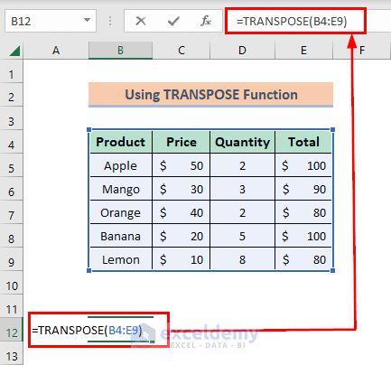
- The table is transposed now. See the result below.
![]()
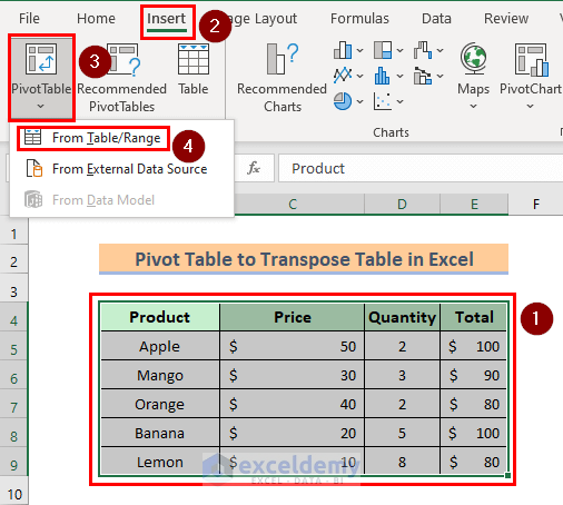
Method 3 – Transposing a Table Using Excel Pivot Table
STEPS:
- Select the whole table.
- Go to the Insert menu ribbon.
- Pick the Pivot Table option. A box will pop up.
- Select Existing Worksheet. Or you can select the other option if you want it in a new sheet.
- Pick the location now. Here I have chosen cell B12.
- Press OK, and a Pivot Table field will appear.
![]()
- Mark all the fields available. The Pivot table will be completed.
![]()
- Go to the bottom of the Pivot Table field.
- Press the Product menu and select Move to Column Labels.
![]()
- Press the Values menu and select Move to Row Labels.
![]()
- The Pivot Table has been transposed.
![]()
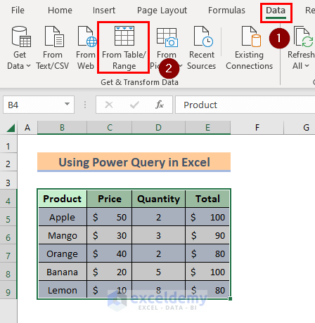
Method 4 – Applying Excel Power Query to Transpose a Table
STEPS:
- Select the whole dataset.
- Go to the Data ribbon.
- Select From Table/Range.
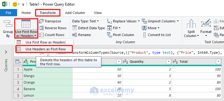
- In the Power Query Editor, go to the Transform ribbon.
- Select Use Headers as First Row.
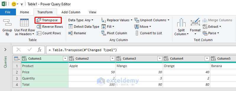
- Press Transpose option.
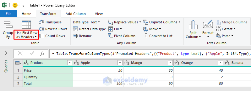
- Select Use First Row as Headers.
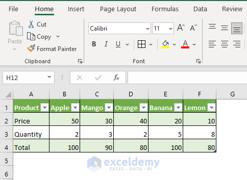
- Go to File menu.
- Press Close & Load.

- The table is transposed now, see the image below.
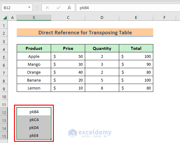
Method 5 – Using Direct Cell Reference for Transposing a Table
STEPS:
- As we want to convert Row 4 to a column, we’ll use the row’s cell references along a new column with some same unique characters before the cell references. We used “pk”.
- Select the new range of cells.
- Click and hold the bottom right corner of the border and drag it to the right until it completes 6 columns. We had 6 rows.
- Select the whole new cells.
- Press Ctrl + H. A dialog box named Find and Replace will open up.
- Type pk in the Find What box and type = in the Replace with box.
- Press Replace All button.
![]()
- Our operation is done, see the screenshot below for the outputs.
![]()
Download Practice Book
Download the Excel workbook that we’ve used to prepare this article.
Related Articles
- Data clean-up techniques in Excel: Changing vertical data to horizontal data
- How to Swap Rows in Excel (2 Methods)
- Convert Columns to Rows in Excel (2 Methods)
- How to Transpose Rows to Columns Using Excel VBA (4 Ideal Examples)
- Excel Transpose Formulas Without Changing References (4 Easy Ways)

