Transposing data means data in Excel’s rows are shifted into Excel’s columns, whether auto-update is necessary or not. Transposing with formulas is the same as transposing data. But it requires extra effort in the case of transposing formulas without changing references. In this article, we’ll demonstrate 5 easy and different approaches to transpose data with formulas without changing the references in Excel.
Download Practice Workbook
You may download the following Excel workbook for better understanding and practice.
5 Easy Ways to Transpose with Formulas Without Changing References in Excel
Suppose, we are using a sheet of Employee Salary Information. This dataset includes the Name, and their corresponding Salary, Allowances, and Total in columns B, C, D, and E respectively.
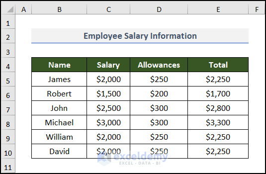
Note: This is a basic dataset to keep things simple. In a practical scenario, you may encounter a much larger and more complex dataset.
Now, we’ll use this dataset to transpose data with formulas in various ways without changing references in Excel.
Not to mention, here, we have used the Microsoft Excel 365 version, you may use any other version according to your convenience. Please leave a comment if any part of this article does not work in your version.
1. Using TRANSPOSE Function
In our first method, we’ll get help from the TRANSPOSE function. This function needs only one argument to accomplish its task. That’s the array argument. Let’s use the function to do our task. Just follow these simple steps below.
📌 Steps:
- At the very beginning, select cell B12 and enter the following formula.
=TRANSPOSE(B4:E10)In this case, B4:E10 represents the range of the whole dataset.
- Then, press ENTER.
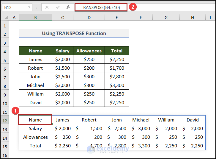
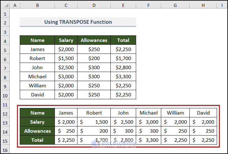
But the formatting won’t come automatically this way. In this situation, we have to do it manually. So, here’s the final look after applying the same formatting as the original dataset.
Read More: How to Transpose in Excel VBA (3 Methods)
2. Utilizing INDIRECT Function
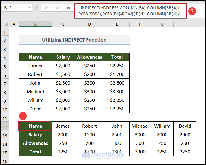
From the heading, you obviously get a hint that we are going to use the INDIRECT function here. But, we’ll combine ADDRESS, COLUMN, and ROW functions in the formula as well. Let’s see it in action.
📌 Steps:
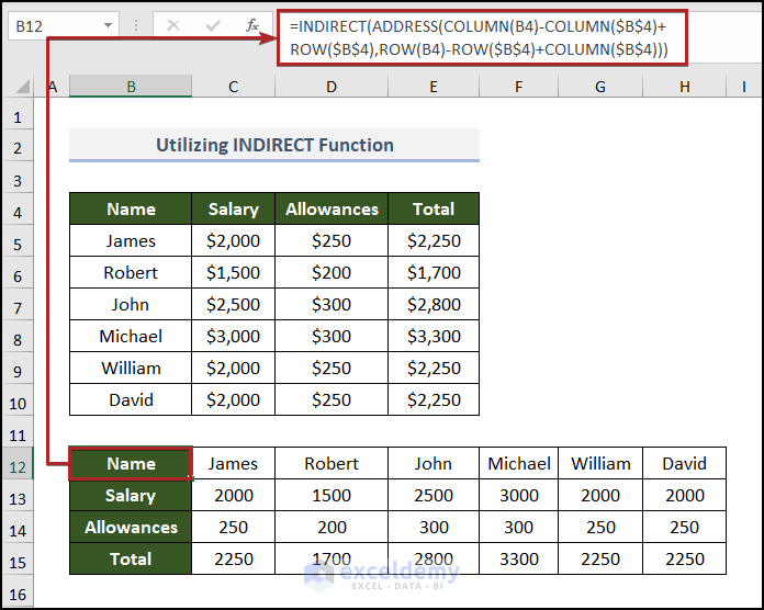
- Firstly, go to cell B12 and insert the formula below.
=INDIRECT(ADDRESS(COLUMN(B4)-COLUMN($B$4)+ROW($B$4),ROW(B4)-ROW($B$4)+COLUMN($B$4)))Formula Breakdown
- In the first argument of the ADDRESS function, “COLUMN(B4) – COLUMN($B$4) + ROW($B$4)” defines the row_num by converting the column number of cell B4.
- Output → 4
- Similarly, in the second argument, “ROW(B4) – ROW($B$4) + COLUMN($B$4)” defines the col_num by converting the row number of cell B4.
- Output → 2
- Then, hit the ENTER key.
Read More: How to Transpose a Table in Excel (5 Suitable Methods)
Similar Readings
- How to Transpose Duplicate Rows to Columns in Excel (4 Ways)
- Excel Power Query: Transpose Rows to Columns (Step-by-Step Guide)
- How to Transpose Rows to Columns Using Excel VBA (4 Ideal Examples)
- Transpose Multiple Columns into One Column in Excel (3 Handy Methods)
- Convert Columns to Rows in Excel Using Power Query
3. Incorporating INDEX Function
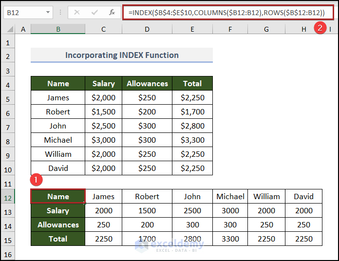
In this method, we’ll integrate the INDEX function with the ROWS and COLUMNS functions to transpose the data in Excel. Let’s explore the method sequentially.
📌 Steps:
- Initially, select cell B12 and write down the following formula in the Formula Bar.
=INDEX($B$4:$E$10,COLUMNS($B12:B12),ROWS($B$12:B12))Formula Breakdown
- COLUMNS($B12:B12) → the COLUMNS function returns the number of columns in the array $B12:B12.
- Output → 1
- ROWS($B$12:B12) → the ROWS function returns the total number of rows in the array $B$12:B12.
- Output → 1
- INDEX($B$4:$E$10,COLUMNS($B12:B12),ROWS($B$12:B12)) becomes INDEX($B$4:$E$10,1,1).
- INDEX($B$4:$E$10,1,1) → the INDEX function returns the value of the intersection of this row_num and col_num in the B4:E10 array.
- Output → Name
- After that, press the ENTER key.
Read More: Conditional Transpose in Excel (2 Examples)
4. Employing OFFSET Function
When you have a tool like Microsoft Excel, you can effortlessly perform such a task in different manners. You could also use the OFFSET function. So, let’s see the process in detail.
📌 Steps:
- Firstly, select cell B12 and put down the following formula.
=OFFSET($B$4,COLUMN()-COLUMN($B$12),ROW()-ROW($B$12))Formula Breakdown
- COLUMN()-COLUMN($B$12) → the COLUMN function returns the column number of the reference cell.
- Output → 0
- ROW()-ROW($B$12) → the ROW function returns the row number of the reference cell.
- Output → 0
- OFFSET($B$4,COLUMN()-COLUMN($B$12),ROW()-ROW($B$12)) becomes OFFSET($B$4,0,0).
- OFFSET($B$4,0,0) → returns a section from a data set with a specific height and a specific width, situated at a specific number of rows down and a specific number of columns right from a given cell reference.
- Output → Name
- Later, press ENTER.

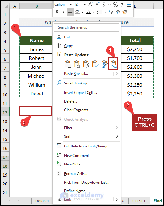
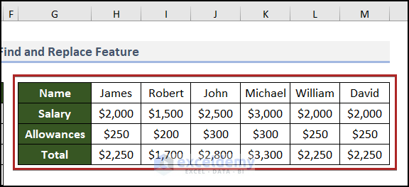
5. Applying Find and Replace Feature
Last but not least, we will employ the Find and Replace feature of Excel to execute the task. Let’s explore the method step-by-step.
📌 Steps:
- Primarily, select cells in the B4:E10 range.
- Then, press CTRL+C on the keyboard.
- After that, click on cell B12 and right-click on the cell.
- From the context menu, select the Paste Link (N) option.
Immediately, the output becomes visible in the B12:E18 range.
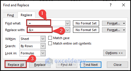
- While keeping it highlighted, press CTRL + H on your keyboard.
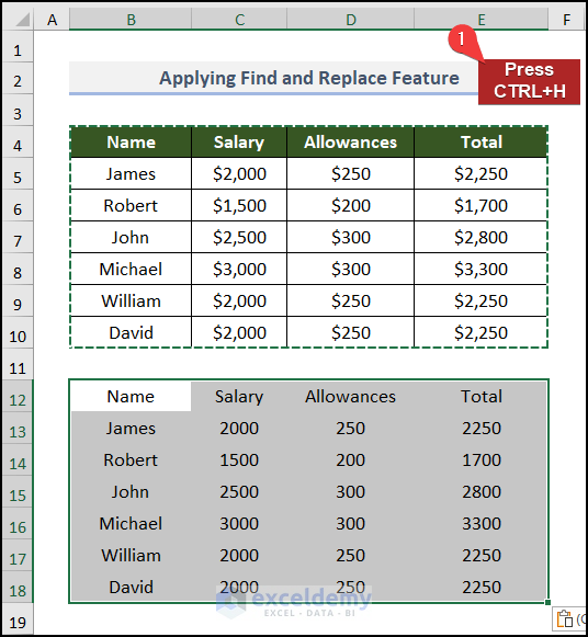
Instantly, the Find and Replace dialog box will open up.
- In the Find what box, write down =.
- Contrarily, write down &= in the Replace with box.
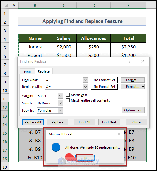
- Lastly, click on the Replace All button.
Just after that, a new MsgBox pops up.
- Here, click OK to neglect it.
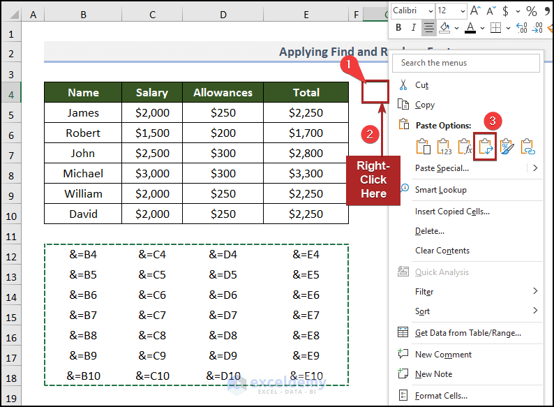
- At this time, highlight the whole range (B12:E18).
- Then, press CTRL + C to copy the data.

- Correspondingly, go to cell G4 where we want the final transposed output.
- After that, right-click here.
- Next, click on the Transpose (T) icon from the Paste Options.
- As the transposed data gets laid in the G4:M7 range, press CTRL + H again.

- Again, write down “&=” in the Find what box of the Find and Replace dialog box.
- In the Replace with box, put down “=”.
- At last, click on the Replace All button.
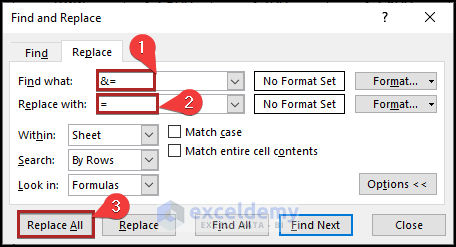
Finally, it’s done. All the columns and rows get transposed with formulas.
Practice Section
For doing practice by yourself, we have provided a Practice section like the one below on each sheet on the right side. Please do it yourself.

Conclusion
This article explains how to transpose with formulas without changing references in Excel in a simple and concise manner. Don’t forget to download the Practice file. Thank you for reading this article. We hope this was helpful. Please let us know in the comment section if you have any queries or suggestions. Please visit our website, ExcelDemy, a one-stop Excel solution provider, to explore more.
Related Articles
- How to Transpose Every n Rows to Columns in Excel (2 Easy Methods)
- Excel VBA: Transpose Multiple Rows in Group to Columns
- How to Transpose Rows to Columns Based on Criteria in Excel
- Reverse Transpose in Excel (3 Simple Methods)
- How to Transpose Rows to Columns in Excel (5 Useful Methods)
- VBA to Transpose Array in Excel (3 Methods)

