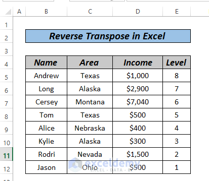
Dataset Overview
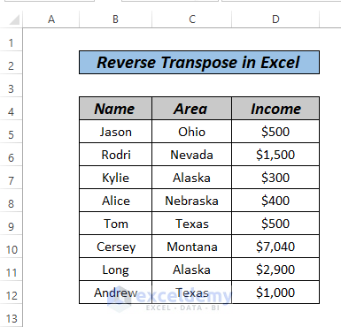
We’ll work with a sample dataset containing columns for Name, Age, Gender, and Monthly Income.
Method 1 – Reverse Transpose Using Sort
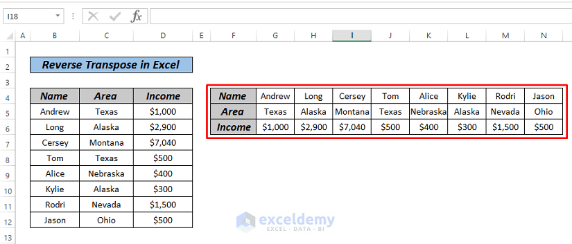
- Copy the entire dataset and paste it as values in cell F4.
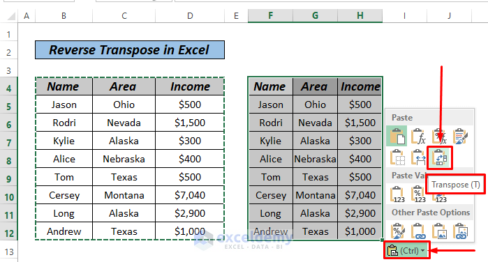
- Click on Transpose (as shown in the image).
![]()
However, this won’t give us the desired result; we want Andrew at the top of the list.
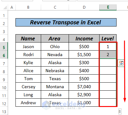
- Add an extra column called Level and fill it using the AutoFill option.
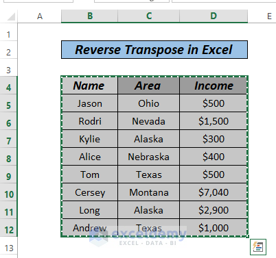
- Select the data (including the header) and go to the Data tab and select Sort.
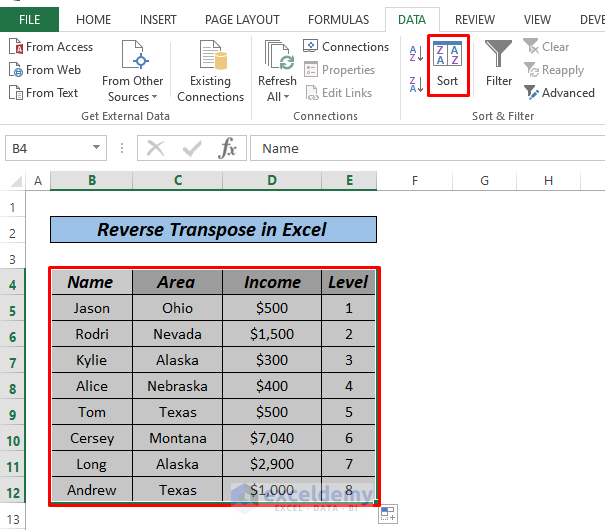
- In the dialog box, choose Level and sort it from Largest to Smallest.
![]()
- Now our dataset should look like the following image:
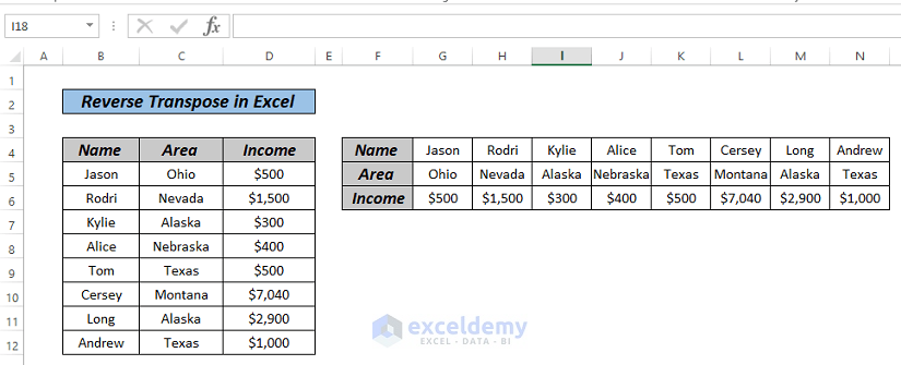
- Delete the Level column and transpose the data again.
Read More: Excel Paste Transpose Shortcut: 4 Easy Ways to Use
Method 2: Reverse Transpose Using Transpose Function
- Transpose the data using Paste Special:
- Select the data range and press CTRL+C.
- Click anywhere and press CTRL+ALT+V to open the dialog box.
![]()
- Choose Transpose and click OK.
Although this won’t give us the desired result, we’ll need these border areas later.
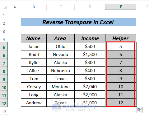
- Add a Helper column with the formula:
=ROW()![]()
- Press ENTER key and drag it down to AutoFill the rest of the series (indicating row numbers).
- Select the dataset. go to the Data tab and select Sort.
![]()
- Sort the Helper column from Largest to Smallest.
![]()
- Our data should resemble the following image.
![]()
- Select the previously transposed data, press Delete, then enter the following formula:
=TRANSPOSE(B4:E12)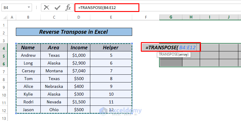
- Press ENTER. If you’re using a lower version of Excel (before 2019), use CTRL+SHIFT+ENTER.
![]()
Similar Readings
- Excel Power Query: Transpose Rows to Columns (Step-by-Step Guide)
- How to Transpose Rows to Columns Using Excel VBA (4 Ideal Examples)
- Transpose Multiple Columns into One Column in Excel (3 Handy Methods)
- How to Swap Rows in Excel (2 Methods)
- How to Change Vertical Column to Horizontal in Excel
Method 3: Using INDIRECT Function to Reverse Transpose
- We’ll start by transposing the data (as shown in the image).

- Click on cell G3 and enter the formula:
COLUMN()![]()
- Drag right and use AutoFill to complete the series.
![]()
- In column P, type the numbers 4, 5, and 6 (indicating column and row numbers).
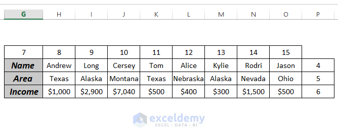
- Click on cell G7 and enter the formula:
=MAX(G3:O3)![]()
- Press ENTER.
![]()
- In cell H7, enter the formula:
=G7-1- Press Enter and AutoFill the rest of the series.
![]()
- In another cell, enter the formula:
=INDIRECT(ADDRESS($P4,G$7))![]()
- Press ENTER and fill the rest of the series by dragging.
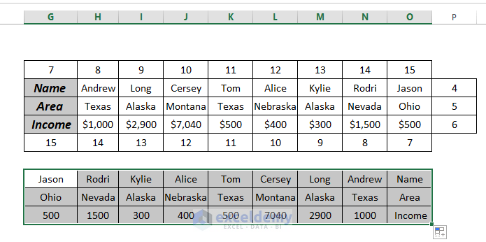
The ADDRESS function provides the cell location based on the given row and column numbers. For example, ADDRESS($P4,G$7) yields the output $O$4. The INDIRECT function retrieves the value from that cell, which in this scenario would be Jason.
Read More: How to Transpose Rows to Columns Based on Criteria in Excel (2 Ways)
Practice Section
We’ve attached a practice workbook for you to practice these methods.
![]()
Download Practice Workbook
You can download the practice workbook from here:
Related Articles
- How to Transpose Duplicate Rows to Columns in Excel (4 Ways)
- How to Transpose Every n Rows to Columns in Excel (2 Easy Methods)
- Convert Columns to Rows in Excel Using Power Query
- How to Convert Columns to Rows in Excel Based On Cell Value
- VBA to Transpose Multiple Columns into Rows in Excel (2 Methods)
- How to Convert Column to Comma Separated List With Single Quotes

