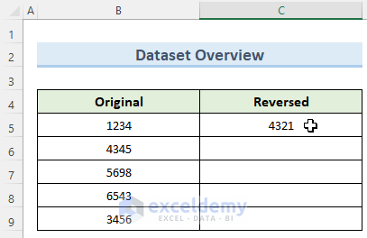
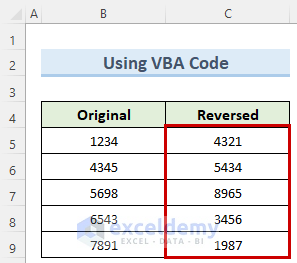
Only 4-digit numbers were used.
Example 1. Combining the SUM and the VALUE Functions
Steps:
- Go to C5 and enter the formula:
=RIGHT(SUM(VALUE(MID(B5&"1",ROW(INDIRECT("1:"&LEN(B5&"1"))),1))*10^(ROW(INDIRECT("1:"&LEN(B5&"1")))-1)),LEN(B5))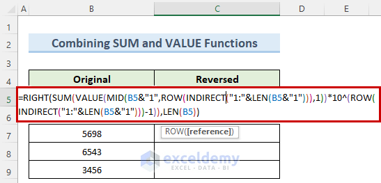
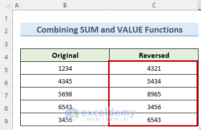
- Press Enter and copy the formula to the other cells using the Fill handle.
- The reversed numbers will be displayed.
Formula Breakdown
- LEN(B5): counts the number of characters and returns 4.
- LEN(B5&”1″): adds a 1 to the number and returns 5.
- INDIRECT(“1:”&LEN(B5&”1”)): references rows 1 to 5.
- ROW(INDIRECT(“1:”&LEN(B5&”1”))): returns the referenced row numbers.
- 10^(ROW(INDIRECT(“1:”&LEN(B5&”1”)))-1): generates the numbers 1, 10, 100, 1000 and 10000 in a column.
- MID(B5&”1″,ROW(INDIRECT(“1:”&LEN(B5&”1”))),1): Returns the numbers 1, 2, 3, 4 and 1 in a column.
- VALUE(MID(B5&”1″,ROW(INDIRECT(“1:”&LEN(B5&”1”))),1))*10^(ROW(INDIRECT(“1:”&LEN(B5&”1”)))-1): Returns 1, 20, 300, 4000 and 10000 in a column.
- SUM(VALUE(MID(B5&”1″,ROW(INDIRECT(“1:”&LEN(B5&”1”))),1))*10^(ROW(INDIRECT(“1:”&LEN(B5&”1”)))-1)): Sums all the values in the column and returns 14321.
- RIGHT(SUM(VALUE(MID(B5&”1″,ROW(INDIRECT(“1:”&LEN(B5&”1”))),1))*10^(ROW(INDIRECT(“1:”&LEN(B5&”1”)))-1)),LEN(B5)): Returns 4321 from the sum.
Read More: How to Paste in Reverse Order in Excel
Example 2. Using the SUMPRODUCT Function
Steps:
- Double-click C5 and enter the formula below:
=RIGHT(SUMPRODUCT(VALUE(MID(B5&"1",ROW(INDIRECT("1:"&LEN(B5&"1"))),1))*10^(ROW(INDIRECT("1:"&LEN(B5&"1")))-1)),LEN(B5))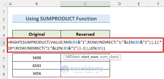
- Press Enter and copy the formula to the other cells using the Fill handle.
- All numbers are in reverse order.

Formula Breakdown
- SUMPRODUCT(VALUE(MID(B5&”1″,ROW(INDIRECT(“1:”&LEN(B5&”1”))),1))*10^(ROW(INDIRECT(“1:”&LEN(B5&”1”)))-1)): adds all values in the column and returns 14321.
- RIGHT(SUMPRODUCT(VALUE(MID(B5&”1″,ROW(INDIRECT(“1:”&LEN(B5&”1”))),1))*10^(ROW(INDIRECT(“1:”&LEN(B5&”1”)))-1)),LEN(B5)): returns 4321 from the sum.
Example 3 – Utilizing the TEXTJOIN Function
Steps:
- Select C5 and enter the following formula:
=TEXTJOIN("",1,MID(B5,{10,9,8,7,6,5,4,3,2,1},1))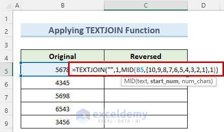
- Press Enter and copy the formula to the other cells using the Fill handle.
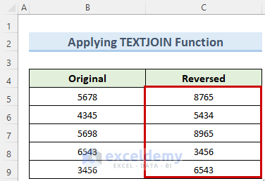
- All numbers are in reverse order.
Formula Breakdown
- MID(B5,{10,9,8,7,6,5,4,3,2,1},1): places each number in 1234 in different cells in a reversed order.
- TEXTJOIN(“”,1,MID(B5,{10,9,8,7,6,5,4,3,2,1},1)): joins the numbers in a cell in reverse order.
Example 4 – Reverse a Number Using a Dynamic Array
Steps:
- Select C5 and enter the following formula:
=TEXTJOIN("",1,MID(B5,ABS(ROW(INDIRECT("1:"&LEN(B5)))-(LEN(B5)+1)),1))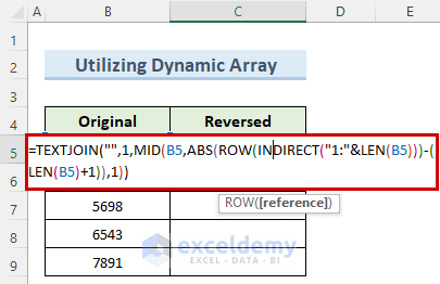
- Press Enter and copy the formula to the other cells using the Fill handle.
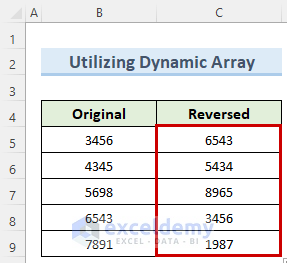
- All numbers are in reverse order.
Formula Breakdown
- LEN(B5)+1: returns number 5.
- ABS(ROW(INDIRECT(“1:”&LEN(B5)))-(LEN(B5)+1)): reverses 1234 and places it in a column with each character in a different cell.
- TEXTJOIN(“”,1,MID(B5,ABS(ROW(INDIRECT(“1:”&LEN(B5)))-(LEN(B5)+1)),1)): Joins the numbers in a cell in reverse order.
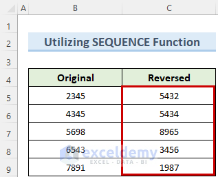
Example 5. Applying the SEQUENCE Function to Reverse a Number
Steps:
- Select C5 and enter the following formula:
=TEXTJOIN("",1,MID(B5,SEQUENCE(LEN(B5),,LEN(B5),-1),1))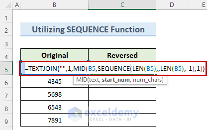
- Press Enter and copy the formula to the other cells using the Fill handle.
- All numbers are in reverse order.
Formula Breakdown
- SEQUENCE(LEN(B5),,LEN(B5),-1): places 4321 in column 4
- TEXTJOIN(“”,1,MID(B5,SEQUENCE(LEN(B5),,LEN(B5),-1),1)): joins the numbers in a cell in reverse order.
Read More: How to Reverse a String in Excel
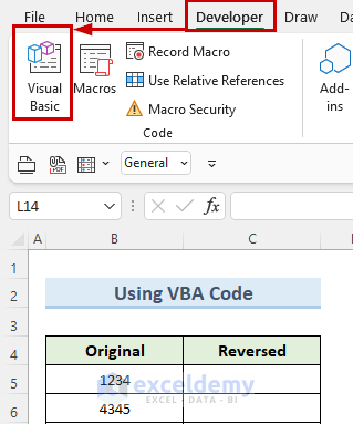
Example 6 – Reversing a Number in Excel Using a VBA Code
Steps:
- Go to the Developer tab and click Visual Basic.
- In the VBA window, click Insert and choose Module.
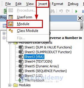
- In the module window, enter the code below:
Public Sub Reverse()
Dim sResult As String
sResult = StrReverse("1234")
Range("C5").Value = sResult
End Sub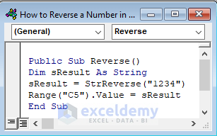
- In the Developer tab, click Macros.
- In the Macro window, select the macro and click Run.
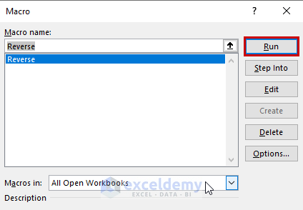
- The VBA code will generate the reverse order of all numbers.
Read More: How to Use Excel VBA to Reverse String
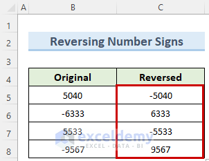
How to Reverse Number Signs (Positive or Negative) in Excel
Steps:
- Click C5 and enter the following formula:
=(-1)*B5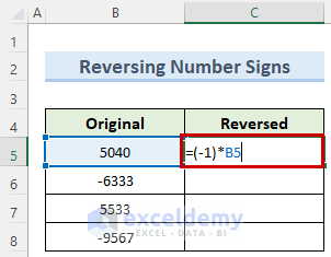
- Press Enter and copy the formula to the other cells in which you want to reverse signs.
Download Practice Workbook
Download the practice workbook here.
Related Articles
- How to Reverse Names in Excel
- How to Switch First and Last Name in Excel with Comma
- How to Reverse Rows in Excel
<< Go Back to Excel Reverse Order | Sort in Excel | Learn Excel
Get FREE Advanced Excel Exercises with Solutions!
