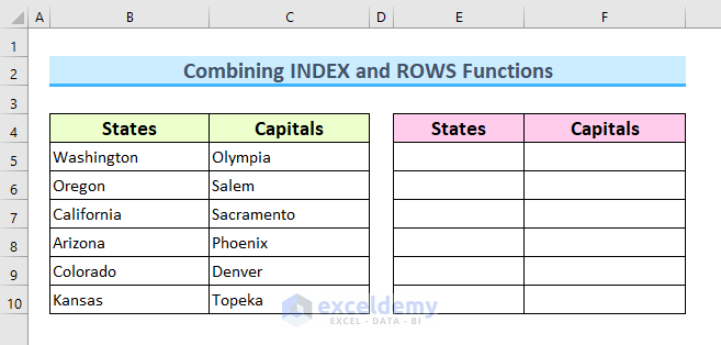
How to Reverse Data in Excel Cell (5 Easy Ways)

Method 1 – Combining INDEX and ROWS Functions to Reverse Data

Create a second data table in your worksheet to see the result after reversing.

Combining INDEX and ROWS Functions to Reverse Data in Excel Cell

Enter the following formula in cell E5 of the new data table.

=INDEX($B$5:$B$10,ROWS(B5:$B$10))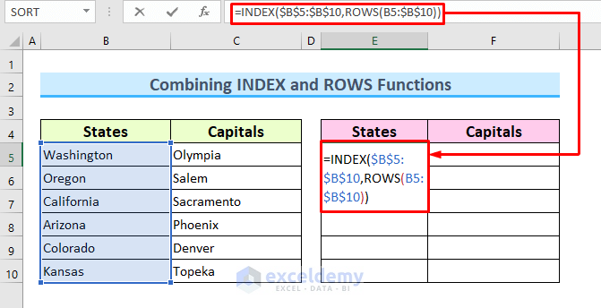

Formula Breakdown

ROWS(B5:$B$10): The ROWS function will show the number of rows that are within this cell range. For our example, there are six rows between cells B5 and B10. As we drag the formula to the lower cells, the number will decrease because we have used a dynamic cell reference.
INDEX($B$5:$B$10,ROWS(B5:$B$10)): the INDEX function will show the result based on the value from the second argument. That means, first it will input the value of the sixth row, then the fifth row, and so on…, thus reversing the data.

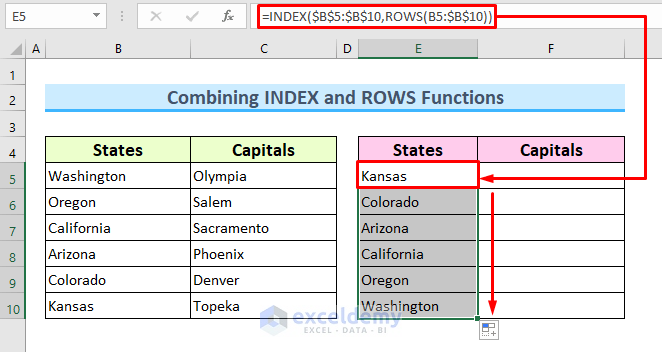
Press Enter to get the last data of column B as the first data of column E.
Use the AutoFill feature to drag the formula to the lower cells.

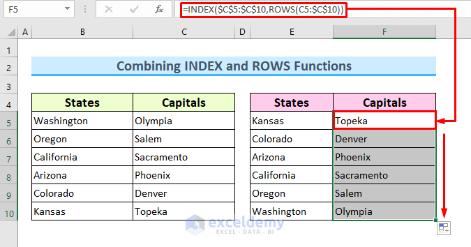
To reverse the name of the capitals, enter the following formula in cell F5.

=INDEX($C$5:$C$10,ROWS(C5:$C$10))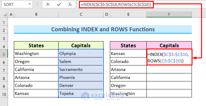

Press Enter and drag the Fill Handle to get results for the lower cells.

Method 2 – Merging SORTBY and ROW Functions to Reverse Data in Excel Cell

Enter the following formula in cell E5.

=SORTBY($B$5:$C$10,ROW(B5:B10),-1)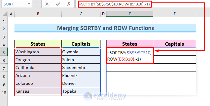

Formula Breakdown

ROW(B5:B10): The ROW function will show the total rows one by one that are in this cell range, that are row 5 to row 10 for our example.
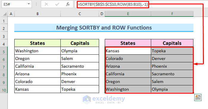
SORTBY($B$5:$C$10,ROW(B5:B10),-1): the SORTBY function will sort the data according to the result of the ROW function. The -1 in the formula will reverse the order and the SORTBY function will fill the data table but in the reverse order.

Press Enter and the formula will reverse the data for the whole data set.

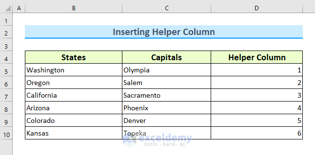
Method 3 – Inserting Helper Column and Helper Row to Reverse Data

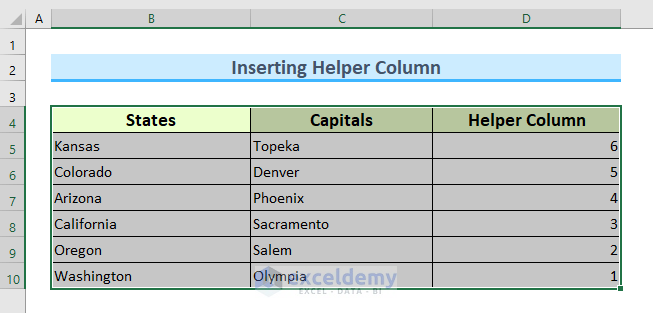
3.1 Inserting Helper Column

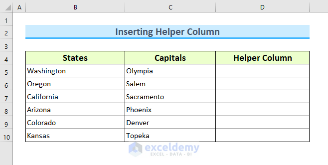
Due to the differences in how the data is organized into columns and rows, reversing data in columns and rows requires a different procedure. To reverse the data in a column, we will insert a helper column.

Make the space for the helper column in column D.

Number the total rows of your data set.
The numbering depends on the reversing requirements.
For our example, we will number from 1 to 6.

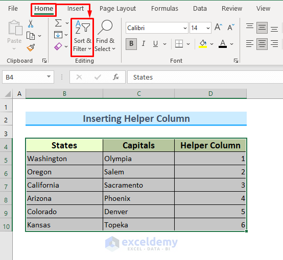
Choose the whole data range, which is B4:D10.
Go to the Home tab of the ribbon.
Select Sort & Filter from the Editing group.

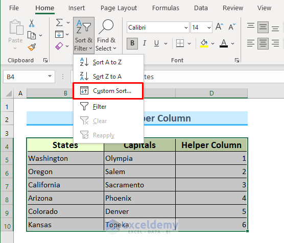
From the Sort & Filter dropdown, choose Custom Sort.

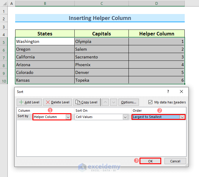
The Sort dialogue box opens.
Under the Sort by dropdown, select Helper Column.
In the Order dropdown, select Largest to Smallest.
Press OK.

The data will be reversed according to the sequence of the helper column.

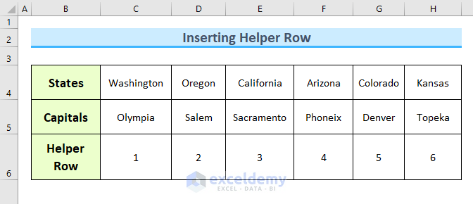
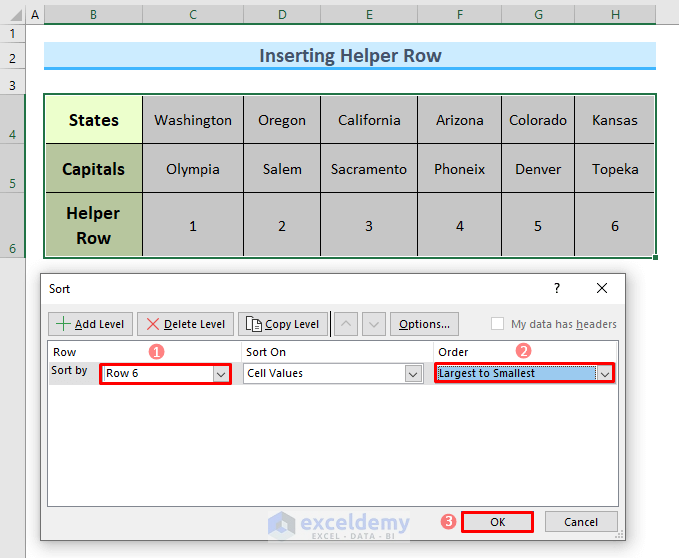
3.2 Inserting Helper Row

The procedure will be different if the data are to be arranged horizontally or in a row. Instead of a helper column, we will insert a helper row.

Insert a new row under the data table to create the helper row.
Name the row and number it according to your desired sequence.

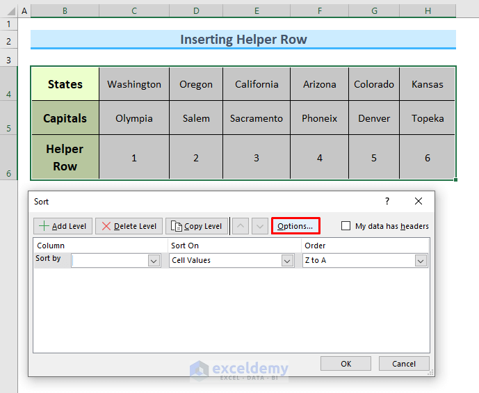
Select the data range from cell B4:H6.
Select the Custom Sort command.
In the Sort dialogue box, choose Options before sorting.

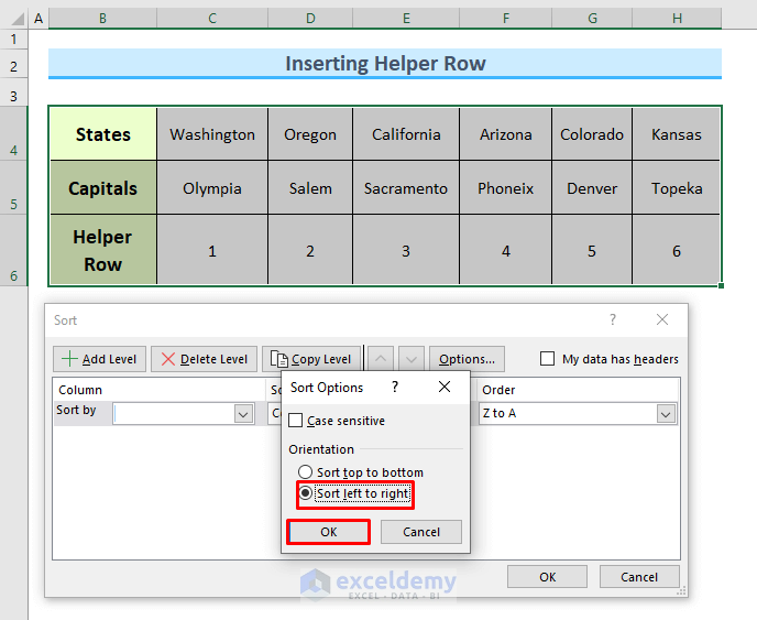
In the Sort Options dialogue box, select Sort left to right for the horizontal sorting.
Press OK.

The Sort dialogue box will pop up.
In the Sort by dialogue box, input the helper row’s row number which is Row 6.
In the Order dropdown, select Largest to Smallest.
Press OK.

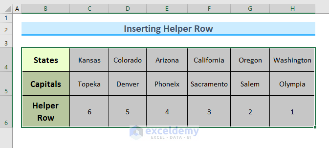
This will reverse the data horizontally.

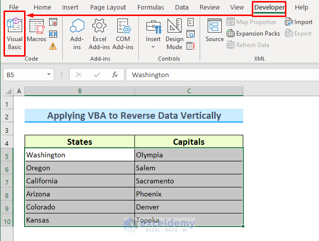
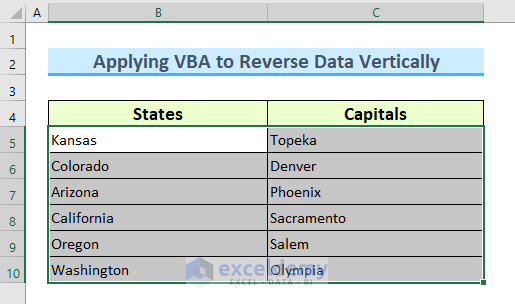
Method 4 – Applying VBA to Reverse Data Vertically in Excel Cell

Select the data range B5:C10.
From the Developer tab, choose Visual Basic.You can press ALT+F11. If you don’t see the Developer tab, follow this link to display the Developer tab on the ribbon.

A VBA window will open.
From the Insert tab, choose Module.

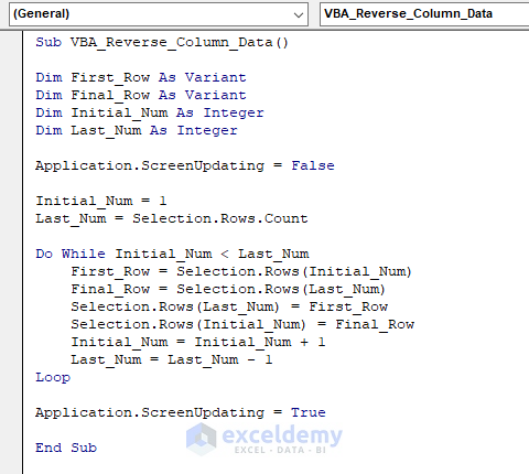
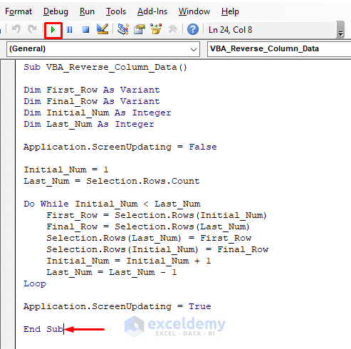
Enter the following code into the module.

Sub VBA_Reverse_Column_Data()
Dim First_Row As Variant
Dim Final_Row As Variant
Dim Initial_Num As Integer
Dim Last_Num As Integer
Application.ScreenUpdating = False
Initial_Num = 1
Last_Num = Selection.Rows.Count
Do While Initial_Num < Last_Num
    First_Row = Selection.Rows(Initial_Num)
    Final_Row = Selection.Rows(Last_Num)
    Selection.Rows(Last_Num) = First_Row
    Selection.Rows(Initial_Num) = Final_Row
    Initial_Num = Initial_Num + 1
    Last_Num = Last_Num - 1
Loop
Application.ScreenUpdating = True
End Sub

VBA Code Breakdown

We are calling the Sub procedure VBA_Reverse_Column_Data.

Sub VBA_Reverse_Column_Data()

We define the variable types.

Dim First_Row As Variant
Dim Final_Row As Variant
Dim Initial_Num As Integer
Dim Last_Num As Integer

We disable the screen updating.

Application.ScreenUpdating = False

We set the initial number as 1 and the last number as the number of rows in the selected range.

Initial_Num = 1
Last_Num = Selection.Rows.Count

We use a loop. We go through the selected range until the initial number is less than the number of rows. It swaps the columns to reverse the data.

Do While Initial_Num < Last_Num
    First_Row = Selection.Rows(Initial_Num)
    Final_Row = Selection.Rows(Last_Num)
    Selection.Rows(Last_Num) = First_Row
    Selection.Rows(Initial_Num) = Final_Row
    Initial_Num = Initial_Num + 1
    Last_Num = Last_Num - 1
Loop

We re-enable the Screen Updating and finish the Sub procedure.

Application.ScreenUpdating = True
End Sub

Save the code in the module and press F5 or the play button to run it, keeping the cursor in the module.

The data in the column will be reversed vertically.

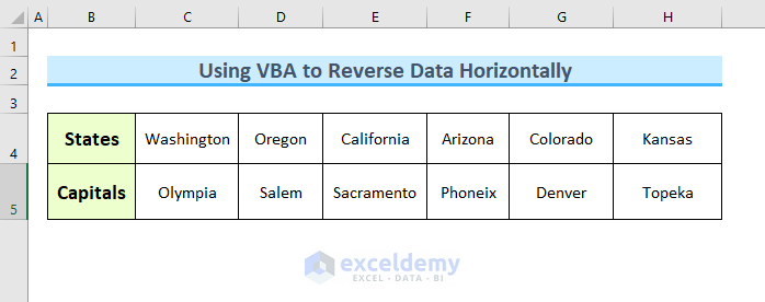
Method 5 – Using VBA to Reverse Data Horizontally

We will use the sample dataset below.

Open the VBA window from the Visual Basic
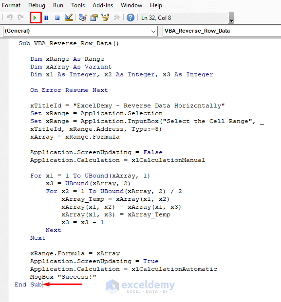
Enter the following code into the module.

 Sub VBA_Reverse_Row_Data()
    Dim xRange As Range
    Dim xArray As Variant
    Dim x1 As Integer, x2 As Integer, x3 As Integer
    On Error Resume Next
    xTitleId = "ExcelDemy - Reverse Data Horizontally"
    Set xRange = Application.Selection
    Set xRange = Application.InputBox("Select the Cell Range", _
    xTitleId, xRange.Address, Type:=8)
    xArray = xRange.Formula
    Application.ScreenUpdating = False
    Application.Calculation = xlCalculationManual
    For x1 = 1 To UBound(xArray, 1)
        x3 = UBound(xArray, 2)
        For x2 = 1 To UBound(xArray, 2) / 2
            xArray_Temp = xArray(x1, x2)
            xArray(x1, x2) = xArray(x1, x3)
            xArray(x1, x3) = xArray_Temp
            x3 = x3 - 1
        Next
    Next
    xRange.Formula = xArray
    Application.ScreenUpdating = True
    Application.Calculation = xlCalculationAutomatic
    MsgBox "Success!"
End Sub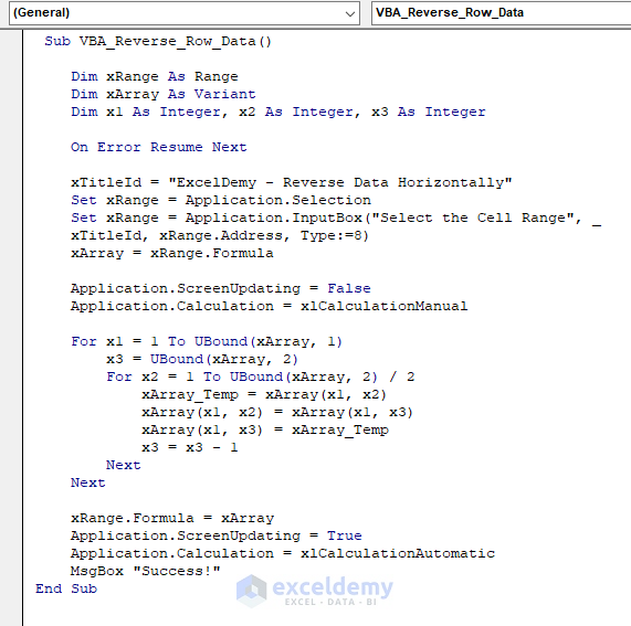

VBA Code Breakdown

We are calling our Sub procedure VBA_Reverse_Row_Data.

Sub VBA_Reverse_Row_Data()

We declare the variable types.

Dim xRange As Range
Dim xArray As Variant
Dim x1 As Integer, x2 As Integer, x3 As Integer

We instruct the code to ignore all errors and continue the loop.

On Error Resume Next

We set the properties of the InputBox.

xTitleId = "ExcelDemy - Reverse Data Horizontally"
Set xRange = Application.Selection
Set xRange = Application.InputBox("Select the Cell Range", _
xTitleId, xRange.Address, Type:=8)

We keep the formula intact.

xArray = xRange.Formula

W set some properties to speed up the code.

Application.ScreenUpdating = False
Application.Calculation = xlCalculationManual

We loop through the range and reverse the data.

For x1 = 1 To UBound(xArray, 1)
x3 = UBound(xArray, 2)
For x2 = 1 To UBound(xArray, 2) / 2
xArray_Temp = xArray(x1, x2)
xArray(x1, x2) = xArray(x1, x3)
xArray(x1, x3) = xArray_Temp
x3 = x3 - 1
Next
Next

We keep the formula intact and set the Application properties to default values and thus completing our code.

xRange.Formula = xArray
Application.ScreenUpdating = True
Application.Calculation = xlCalculationAutomatic
MsgBox "Success!"
End Sub

Save the code in the module.
Keeping the cursor in the module, Run the code.

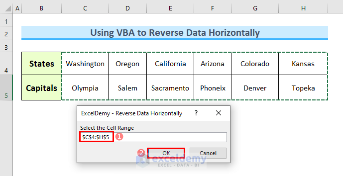
The code will ask for the cell range to reverse the data.
Select the cell range C4:H5 and press OK.

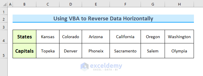
The data arranged horizontally will be reversed.

Download Practice Workbook

Reversing Data.xlsm

<< Go Back to Excel Reverse Order | Sort in Excel | Learn Excel

Get FREE Advanced Excel Exercises with Solutions!