Method 1 – Using Flash Fill Feature to Reverse Names in Excel
Steps:
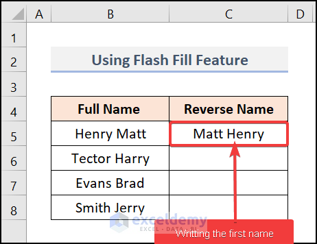
- Enter the first name in your desired order as shown below.
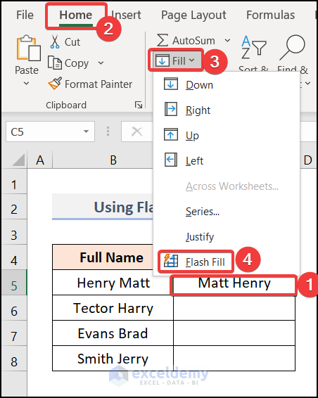
- Select the first cell of the Reverse Name column and go to the Home tab >> Fill drop-down >> Flash Fill.
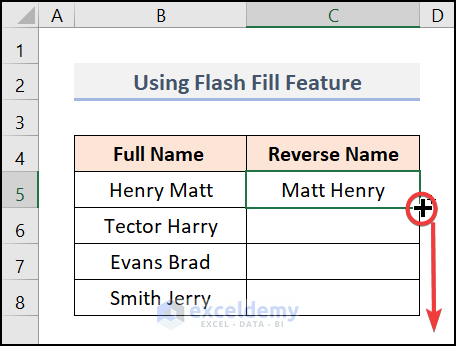
- Click on cell C5 and then drag down the Fill Handle tool for other cells.
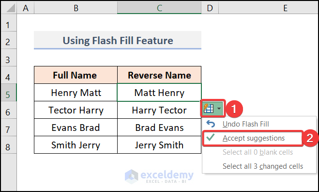
- If you get the desired output, click on the icon shown in the following image and select Accept suggestions.
Method 2 – Reversing Names with MID, SEARCH, and LEN Functions
Steps:
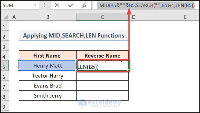
- Select cell C5 and enter the following formula.
=MID(B5&” “&B5,SEARCH(” “,B5)+1,LEN(B5))
The other option is to enter it on the function box.
B5 is the First Name of the employee.
Formula Breakdown:
- LEN(B5) → becomes
- LEN(“Henry Matt”) → The LEN function determines the length of the characters
- Output → 10
- SEARCH(” “,B5) → becomes
- SEARCH(” “,“Henry Matt”) → The SEARCH function finds the position of space in the text Henry Matt
- Output → 6
- SEARCH(” “,B5)+1 → becomes
- 6+1 → 7
- B5&” “&B5 → becomes
- “Henry Matt”&” “&“Henry Matt” → The Ampersand Operator will add up the two texts Henry Matt
- Output → “Henry Matt Henry Matt”
- MID(B5&” “&B5,SEARCH(” “,B5)+1,LEN(B5)) → becomes
- MID(“Henry Matt Henry Matt”,7,10) → 7 is the start number of the characters and 10 is the total number of characters which we will extract using the MID function from the text “Henry Matt Henry Matt”.
- Output → Matt Henry
- MID(“Henry Matt Henry Matt”,7,10) → 7 is the start number of the characters and 10 is the total number of characters which we will extract using the MID function from the text “Henry Matt Henry Matt”.
- “Henry Matt”&” “&“Henry Matt” → The Ampersand Operator will add up the two texts Henry Matt
- SEARCH(” “,“Henry Matt”) → The SEARCH function finds the position of space in the text Henry Matt
- LEN(“Henry Matt”) → The LEN function determines the length of the characters
- Press ENTER.
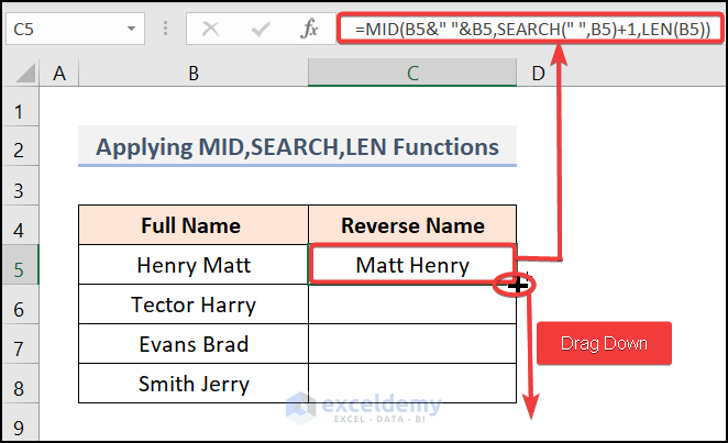
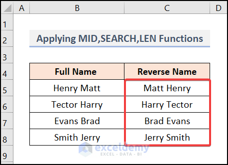
Use the Fill Handle tool for the remaining cells.
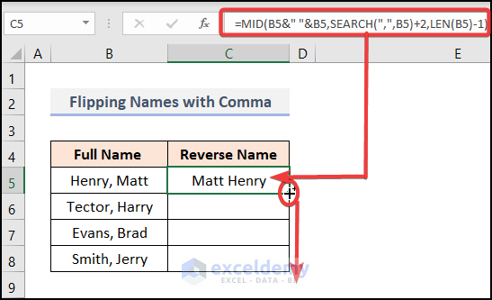
Method 3 – Flipping Names with Comma in Excel
Steps:
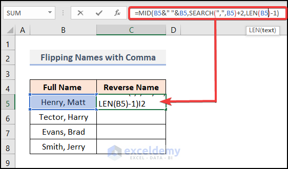
- Select cell C5 and enter the following formula.
=MID(B5&” “&B5,SEARCH(“,”,B5)+2,LEN(B5)-1)
B5 is the First Name of the employee.
Formula Breakdown:
- LEN(B5)-1 → becomes
- LEN((“Henry, Matt”)-1) → The LEN function determines the length of the characters
- Output → 10
- SEARCH(“, “,B5) → becomes
- SEARCH(“, “,“Henry, Matt”) → The SEARCH function finds the position of space in the text Henry Matt
- Output → 6
- SEARCH(” “,B5)+2 → becomes
- 6+2 → 8
- B5&” “&B5 → becomes
- “Henry, Matt”&” “&“Henry, Matt” → The Ampersand Operator will add up the two texts Henry Matt
- Output → “Henry, Matt Henry, Matt”
- =MID(B5&” “&B5,SEARCH(“,”,B5)+2,LEN(B5)-1)→ becomes
- MID(“Henry, Matt Henry, Matt”,8,10) → 8 is the start number of the characters and 10 is the total number of characters which we will extract using the MID function from the text “Henry, Matt Henry, Matt”.
- Output → Matt Henry
- MID(“Henry, Matt Henry, Matt”,8,10) → 8 is the start number of the characters and 10 is the total number of characters which we will extract using the MID function from the text “Henry, Matt Henry, Matt”.
- “Henry, Matt”&” “&“Henry, Matt” → The Ampersand Operator will add up the two texts Henry Matt
- SEARCH(“, “,“Henry, Matt”) → The SEARCH function finds the position of space in the text Henry Matt
- LEN((“Henry, Matt”)-1) → The LEN function determines the length of the characters
- Press ENTER.
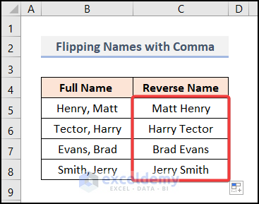
- Use the Fill Handle tool for the remaining cells.
The result will be displayed in the Reverse Name column.
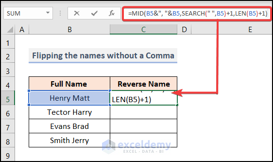
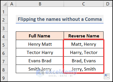
Method 4 – Reversing Names in Excel Without a Comma
Steps:
- Select the cell C5 and enter the following formula.
=MID(B5&”, “&B5,SEARCH(” “,B5)+1,LEN(B5)+1)
B5 is the First Name of the employee.
Formula Breakdown:
- LEN(B5)+1 → becomes
- LEN((“Henry Matt”)+1) → The LEN function determines the length of the characters
- Output → 11
- SEARCH(“, “,B5)+1 → becomes
- SEARCH((“, “, “Henry Matt”)+1) → The SEARCH function finds the position of space in the text Henry Matt
- Output → 6+1→7
- B5&”, “&B5 → becomes
- “Henry Matt”&”,”&“Henry Matt” → The Ampersand Operator will add up the two texts Henry Matt
- Output → “Henry Matt, Henry Matt”
- =MID(B5&” “&B5,SEARCH(“,”,B5)+2,LEN(B5)-1)→ becomes
- MID(“Henry Matt, Henry Matt”,7,11) → 7 is the start number of the characters and 11 is the total number of characters which we will extract using the MID function from the text “Henry Matt, Henry Matt”.
- Output → Matt, Henry
- MID(“Henry Matt, Henry Matt”,7,11) → 7 is the start number of the characters and 11 is the total number of characters which we will extract using the MID function from the text “Henry Matt, Henry Matt”.
- “Henry Matt”&”,”&“Henry Matt” → The Ampersand Operator will add up the two texts Henry Matt
- SEARCH((“, “, “Henry Matt”)+1) → The SEARCH function finds the position of space in the text Henry Matt
- LEN((“Henry Matt”)+1) → The LEN function determines the length of the characters
- Press ENTER.
- Use the Fill Handle tool for the remaining cells.
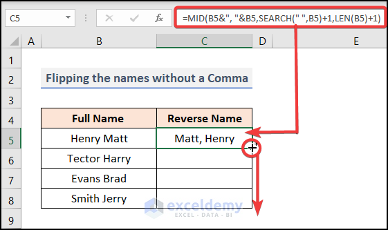
The following result will be displayed.
Read More: How to Reverse a String in Excel
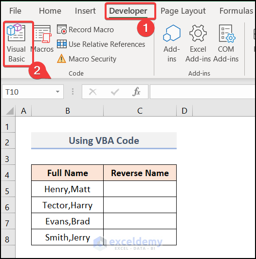
Method 5 – Reversing Names with Excel VBA
Steps:
- Go to the Developer tab >> Visual Basic option.
- Click on the Insert tab and select the Module option.
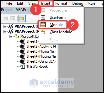
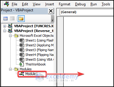
Module 1 will be created where we will insert our code.
- Enter the following VBA code inside the created module
Sub name_flip()
Dim rng As Range
Dim wrk_rng As Range
Dim sym As String
On Error Resume Next
Set wrk_rng = Application.Selection
Set wrk_rng = Application.InputBox("Range", "Exceldemy", wrk_rng.Address, Type:=8)
sym = Application.InputBox("Symbol interval", "Exceldemy", " ", Type:=2)
For Each rng In wrk_rng
    yValue = rng.Value
    name_list = VBA.Split(yValue, sym)
    If UBound(name_list) = 1 Then
        rng.Offset(0, 1) = name_list(1) + sym + name_list(0)
    End If
Next
End Sub name_flip is the sub-procedure name. We have declared rng, wrk_rng as Range, sym as String. 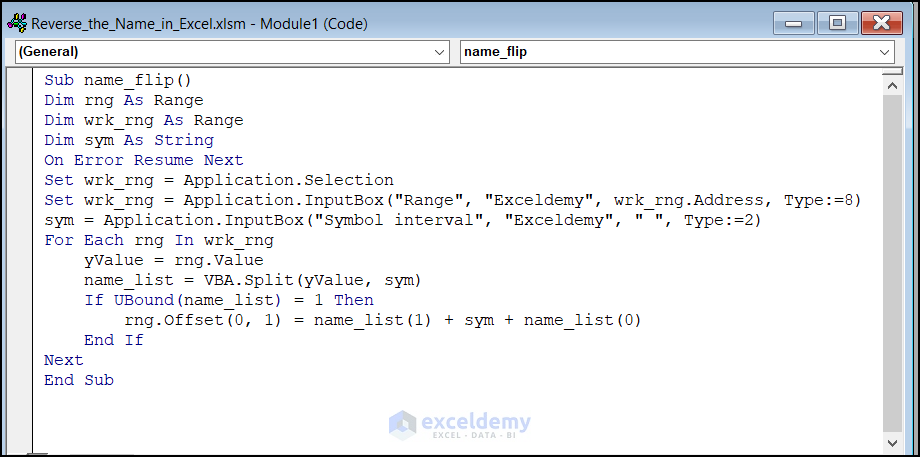
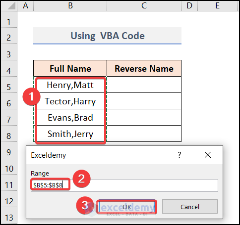
- Run the code by pressing F5.
- In the input box, select all the cells you want to reverse ($B$5:$B$8 is our selected range) and press OK.
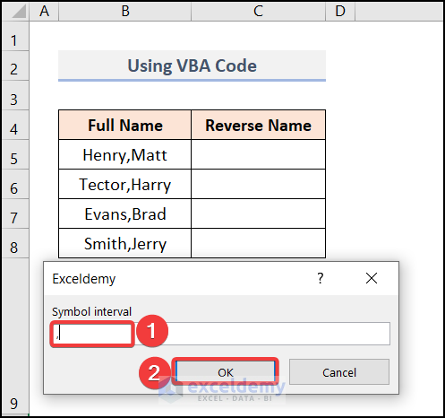
- Another input box will pop up.
- Enter a comma (,) as the symbol for interval and press OK.
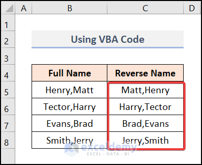
- You will get your result.
Read More: How to Use Excel VBA to Reverse String
Download Practice Workbook
Related Articles
- How to Reverse a Number in Excel
- How to Switch First and Last Name in Excel with Comma
- How to Paste in Reverse Order in Excel
- How to Reverse Rows in Excel
<< Go Back to Excel Reverse Order | Sort in Excel | Learn Excel
Get FREE Advanced Excel Exercises with Solutions!

I Want to Copy many Rows by Selection from one sheet to another sheet using Macro. Is it possible?
Hi, Muhammad! Of course, you can do that. Check this out 🙂
https://www.exceldemy.com/excel-macro-to-copy-and-paste-from-one-worksheet-to-another/#9_VBA_Macro_to_Copy_and_Paste_Selected_Data_from_One_Sheet_to_Another_in_Excel