How to Reverse Data in Excel Chart: 4 Useful Methods

Method 1: Reverse Data in Excel Chart by Formatting Axis

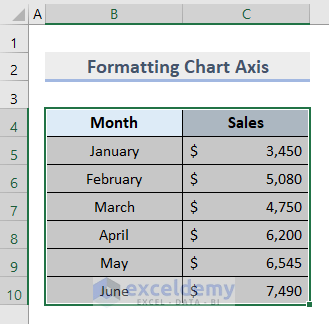
• Select cell range B4:C10.

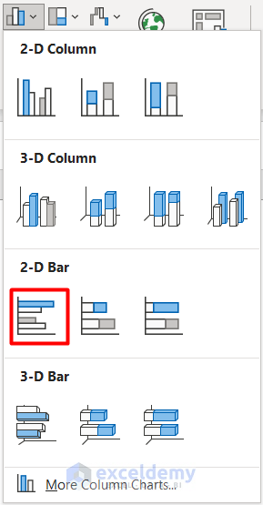
• Go to the Insert tab and click on Bar Chart under the Charts group.

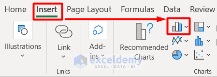
• Select the 2-D Clustered Bar from the drop-down menu.

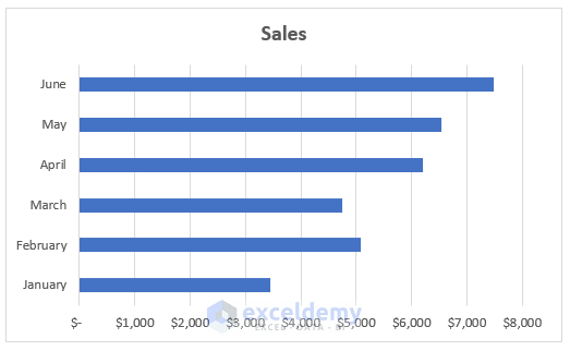
• The chart will look like this:

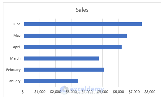
• Reverse the data in this chart.
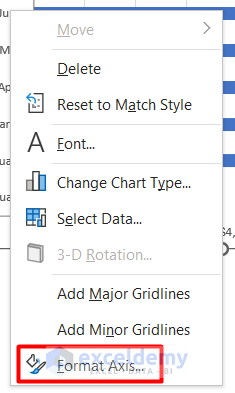
• Right-click on the vertical axis and select Format Axis.

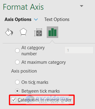
• Mark checked the Category in the reverse order box.

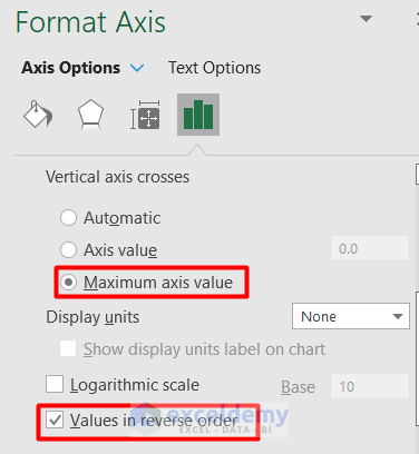
• Open the Format Axis panel for the horizontal axis.
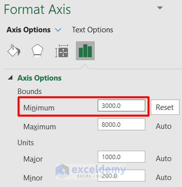
• Select the option Maximum axis value.
• Mark the Values in reverse order box.

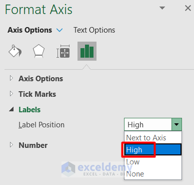
• Make the Label Position as High.

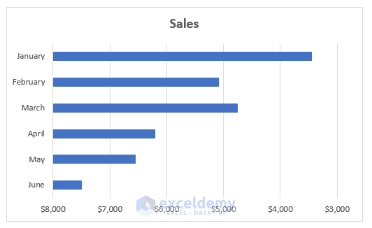
• Set the Minimum value of Bounds at 3000.

• You will successfully reverse data in your Excel chart.

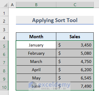
Method 2: Apply Sort Tool for Reversing Data in Excel Chart

• Insert a 2-D Bar Chart like the above with the same dataset.

• Select cell range B5:C10.

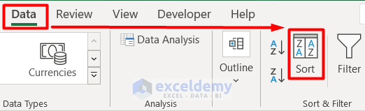
• Go to the Data tab and select Sort under the Sort & Filter group.

• You will see the Sort window.
• Insert Sales and Cell Values as Column and Sort On categories, respectively.
• Set the Order from Largest to Smallest.

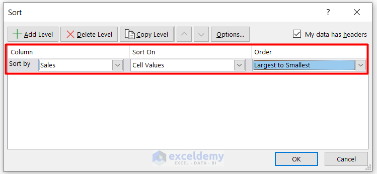
• Press OK.
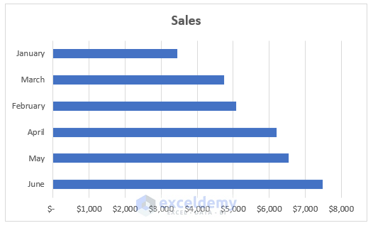
• You will see the chart data has changed automatically.

Method 3: Flip Excel Chart Data Using Select Data Command

• Create the initial chart like before.

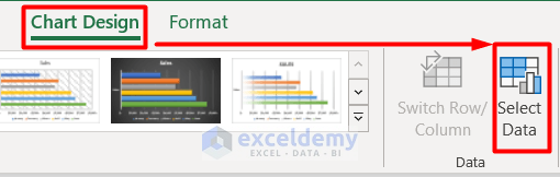
• Select the chart and go to the Chart Design tab.
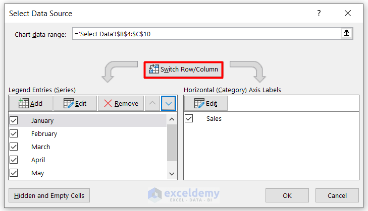
• Click on Select Data under the Data group.

• Reverse the column and row by clicking the Switch Row/Column icon.

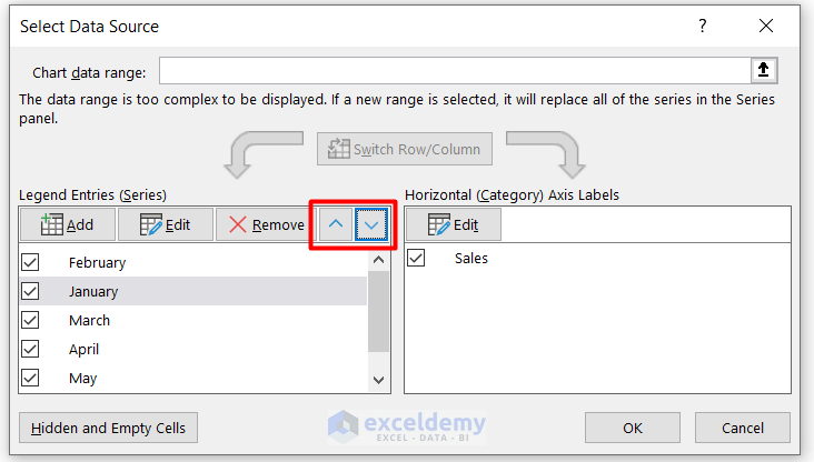
• Use the Move Up and Move Down buttons in the Legend Entries (Series) box to make the position of the values.

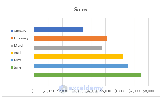
• The reversed data chart is shown in the image below:

Method 4: Insert Excel VBA Code for Reversing Chart Data

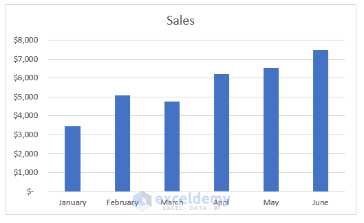
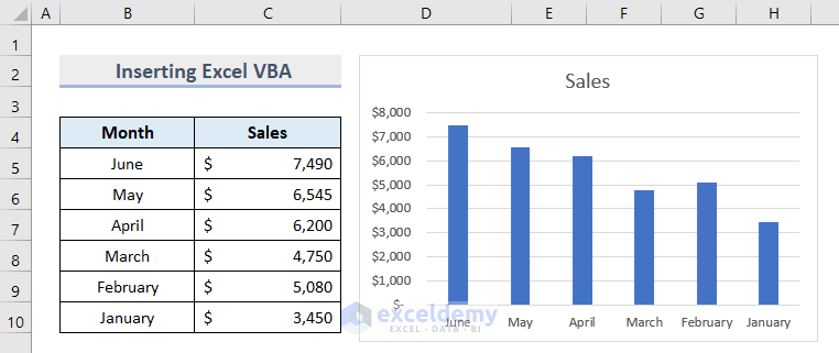
• Insert a 2-D Column Chart based on a similar dataset we described above.

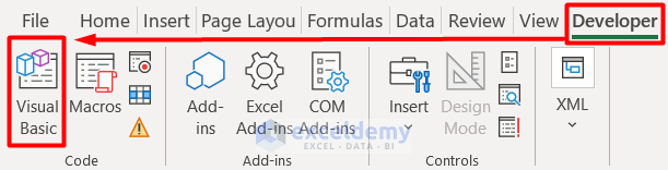
• Go to the Developer tab and select Visual Basic under the Code group.

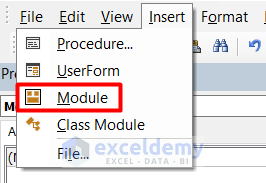
• Select Module from the Insert tab.

• Insert this code on the blank page.

Sub ReverseData()
Dim Tw As Variant
Dim Lw As Variant
Dim SNum As Integer
Dim LNum As Integer
Application.ScreenUpdating = False
SNum = 1
LNum = Selection.Rows.Count
Do While SNum < LNum
Tw = Selection.Rows(SNum)
Lw = Selection.Rows(LNum)
Selection.Rows(LNum) = Tw
Selection.Rows(SNum) = Lw
SNum = SNum + 1
LNum = LNum - 1
Loop
Application.ScreenUpdating = True
End Sub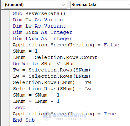

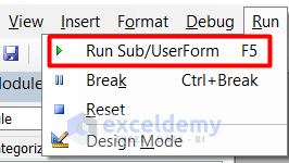
• Click on the Run Sub and press F5 on your keyboard.

• Click on the Run button in the Macros window.

• You will see that the values have turned reverse and the chart also changed in parallel.

Things to Remember

• Prepare your dataset carefully so that it can benefit the process of reversing.
• Make sure there is no blank cell. Otherwise, it will result in false output.
• It is better to keep a copy of the original dataset for future reference.
• You must select the whole dataset before running the VBA code.

Download Practice Workbook

Download this sample file to try at home.

Related Articles

• How to Reverse Data in Excel Cell
• How to Mirror Data in Excel
• How to Reverse Text to Columns in Excel
• How to Reverse Column Order in Excel

<< Go Back to Excel Reverse Order | Sort in Excel | Learn Excel