How to Reverse Column Order in Excel: 4 Useful Methods

Method 1 – Use Sort Feature to Reverse Column Order in Excel

Steps:

• Select the Helper Column.

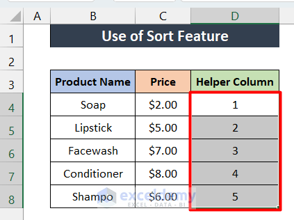
• Go to the Data On the Sort and Filter group, choose Sort Largest to Smallest, shown by the red color box in the figure below.

• After clicking this, a new window will pop up like this below.

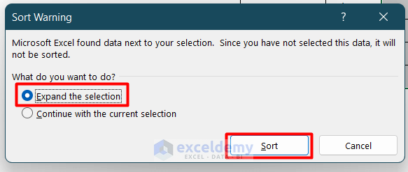
• Choose Expand the selection and click You will get the following result.

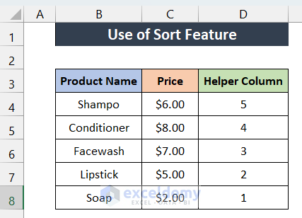
• See that the column order has been reversed. Now Shampo is on the top, and Soap is on the bottom.
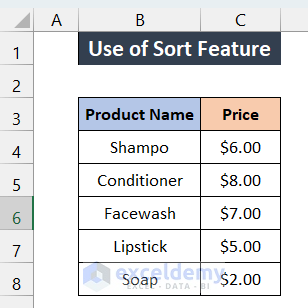
• We don’t need the Helper Column anymore, we can delete the extra column and get our clean result like this below.

Method 2 – Combine SORTBY and ROW Functions to Reverse Column Order in Excel

Another good approach or reverse column in Excel combines the SORTBY and the ROW functions. The ROW function gives an array of row numbers of selected cells. On the other hand, the SORTBY function sorts the contents of a range or array based on the values in a corresponding range or array.

The formula that we will use is below:

• B4: C8 is the array that will be reversed/sorted.
• ROW(B4:B8) will give the row number of product.
• -1 is for sorting the data in descending order.

To apply this formula, follow the steps below.

Steps:

• Let’s create a header column for reversed ordered data like this.

• In cell E4, Input the formula mentioned above.

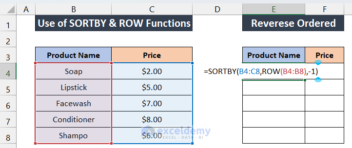
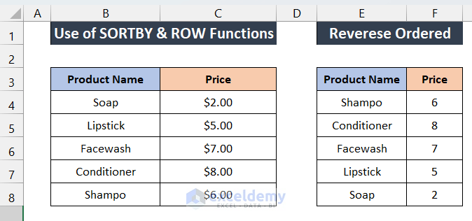
• Click Enter, and you will see the following result.

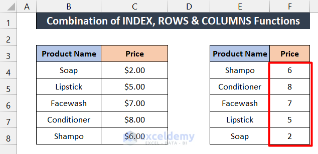
Method 3 – Merge INDEX, ROWS, and COLUMNS Functions to Reverse Column Order

Steps:

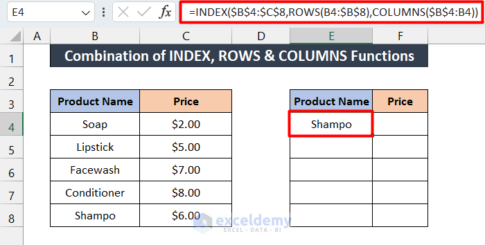
• Copy the two header cells and paste them into cells E3 and F3.

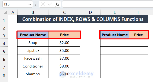
• In E4, Write down the following formula:

• COLUMNS($B$4:B4): Search and return the specified cell reference column number.
• ROWS(B4:$B$8): Looks up and returns the number of rows in each reference or array.
• INDEX($B$4:$C$8,ROWS(B4:$B$8),COLUMNS($B$4:B4)): This will take the whole range of data and then reverse the columns.
• Now press Enter. You will get the following result.

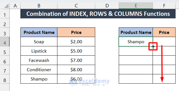
Drag the Fill Handle down to duplicate the formula over the range. To AutoFill the range, double-click on the Plus (+) symbol, as shown in the figure below.

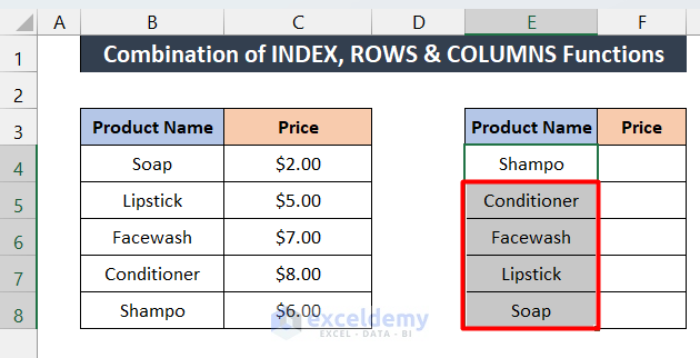
You will see that the cells below have been filled with product names in reversed order.

• To replicate the formula throughout the range, drag the Fill Handle rightwards like below.

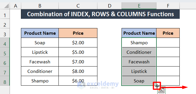
• Now you will see that the Price has also been reversed in the right column.

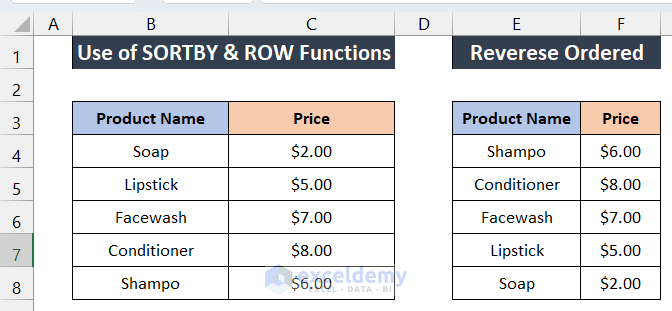
• Like method 2, it also doesn’t give you the cell format. You have to do it manually.

Method 4 – Run a VBA Macro Code to Reverse Column Order

Steps:

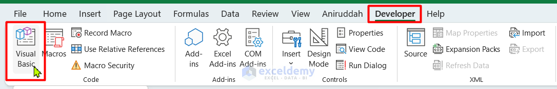
• Go to the Developer tab, and select Visual Basics. You can also press the alt+ f11. If you don’t see the Developer tab, then follow this link to display the Developer tab on the ribbon.

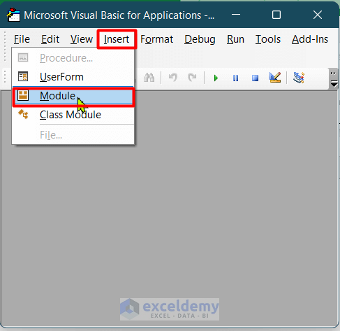
• A new window will pop up. In this window, click on Insert and select Module.

• You will see a window like this.

• Copy the code below and paste it into the window.

 Sub Reverse_Columns()
    Dim Rg As Range
    Dim WRg As Range
    Dim Ar As Variant
    Dim a As Integer, b As Integer, c As Integer
    On Error Resume Next
    xTitleId = "Reverse columns"
    Set WRg = Application.Selection
    Set WRg = Application.InputBox("Range", xTitleId, WRg.Address, Type:=8)
    Ar = WRg.Formula
    Application.ScreenUpdating = False
    Application.Calculation = xlCalculationManual
    For b = 1 To UBound(Ar, 2)
        c = UBound(Ar, 1)
            For a = 1 To UBound(Ar, 1) / 2
                xTemp = Ar(a, b)
                Ar(a, b) = Ar(c, b)
                Ar(c, b) = xTemp
                c = c - 1
            Next
    Next
    WRg.Formula = Ar
    Application.ScreenUpdating = True
    Application.Calculation = xlCalculationAutomatic
End Sub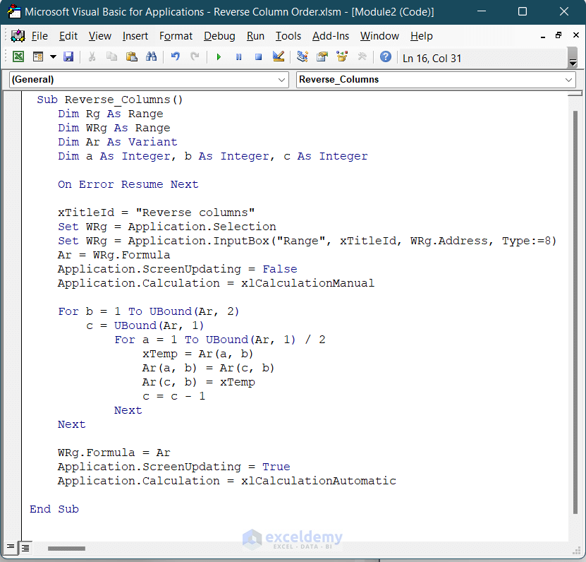

• Run the code by pressing the F5 key. A window will appear like this.

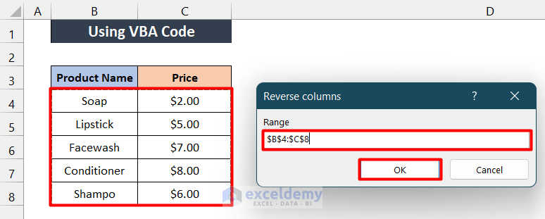
• You must select the cell range from B4 to C8 and click OK. You will get the following result.

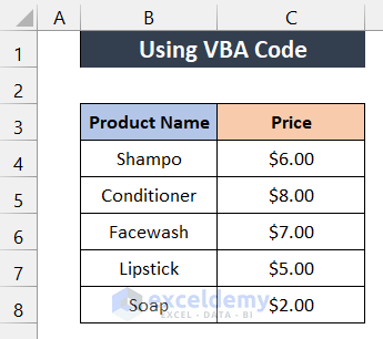
You can see that we have got our desired result. Here Shampo is at the top, and Soap is at the bottom of the list.

Things to Remember

• The first method is the easiest and fastest among the four methods.
• The 2nd and 3rd methods don’t copy the cell format. So you have to manually adjust it.
• If your works require reversing column order frequently, then you should consider the 4th method of using VBA code.

Download Practice Workbook

Download this practice workbook to exercise while you are reading this article.

Related Articles

• How to Reverse Data in Excel Cell
• How to Mirror Data in Excel
• How to Reverse Text to Columns in Excel
• How to Reverse Order of Data in Excel
• How to Reverse Data in Excel Chart

<< Go Back to Excel Reverse Order | Sort in Excel | Learn Excel