How to Mirror Data in Excel: 3 Easy Methods

Method 1 – Link Cells to Mirror Data

Steps:

• First and foremost, click on the B5 cell and insert the following formula.

• Subsequently, hit the Enter button.

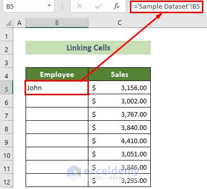
• As a result, you will get the name of the first employee of your dataset.
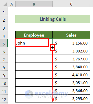
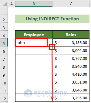
• All other employees, place your cursor in the bottom right position of the B5 cell.
• A black fill handle will appear.
• Drag it below to copy the same formula dynamically.

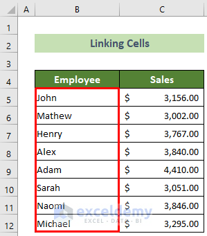
The mirroring would be successful, and you would get the names of the employees. For example, the result would look like this.

Method 2 – Mirror Data Using INDIRECT and ROW Functions

Steps:

• At the very beginning, click on the B5 cell and insert the following formula.

• Hit the Enter button.

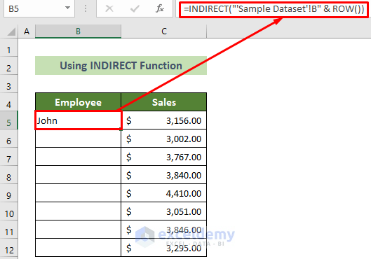
• You will get the name of the first employee from your dataset.
• Place your cursor in the bottom right position of the cell.
• A black fill handle will appear. Drag it below to copy the same formula below.

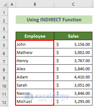
You will be able to mirror data in Excel successfully. The outcome should look like this.

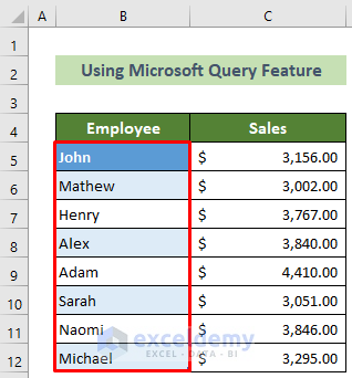
Method 3 – Using Microsoft Query Feature

Steps:

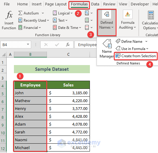
• You need to create a named range of the cells you want to mirror.
• Select the cells B4: B12 >> go to the Formula tab >> Defined Names group >> Create from Selection tool.

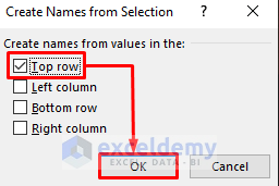
• A window named Create Names from Selection would appear.
• Check the Top Row option here and click the OK button.

• Go to your sheet where you want mirroring to occur.
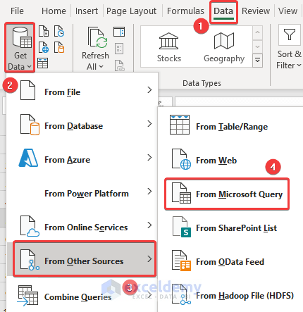
• Go to the Data tab >> Get Data tool >> From Other Sources option >> From Microsoft Query option.

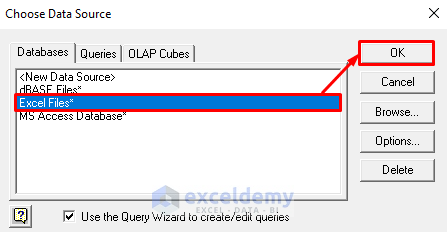
• The Choose Data Source window will appear.
• Choose the Excel Files* option from the Databases tab. Click the OK button.

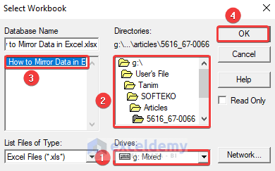
• The Select Workbook window will appear.
• Browse your Excel file from Drive, Directories, and Database Name options. Click the OK button.

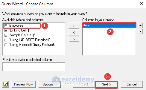
• The Query Wizard – Choose Columns window will arrive.
• Select Employee >> select John >> click the Next button.

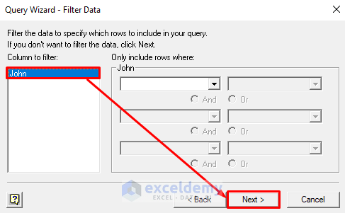
• The Query Wizard – Filter Data window will appear.
• Choose the option John and click the Next button.

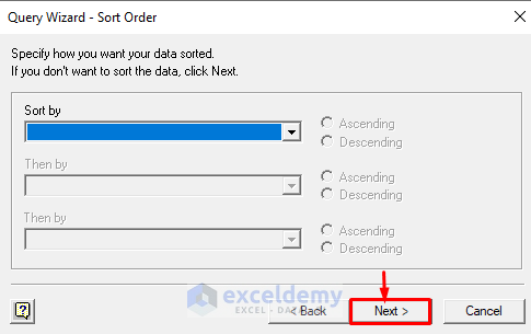
• The Query Wizard – Sort Order window will appear. Click the Next button.

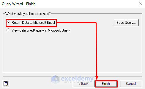
• The Query Wizard – Finish window would appear.
• Choose the first option here and click on the Finish button.

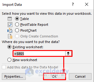
• The Import Data window will appear.
• Wrrite your cell reference where you want to put the mirrored cells (B5 here).
• Click the OK button.

• The mirrored cells would appear as a table.
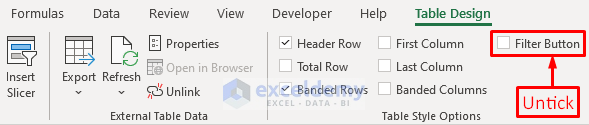
• Go to the Table Design tab >> untick the Filter Button option.

You have successfully mirrored the desired cells in your desired position. The output should look like this.

Things to Remember

Using the Microsoft Query Feature would enable you to mirror data between worksheets. But, the other two ways described here would be able to mirror data between worksheets only.

Download Practice Workbook

You can download our practice workbook here for free!

Related Articles

• How to Reverse Text to Columns in Excel
• How to Reverse Order of Data in Excel
• How to Reverse Column Order in Excel
• How to Reverse Data in Excel Chart

<< Go Back to Excel Reverse Order | Sort in Excel | Learn Excel