Although Excel offers no direct ways to do so, in this article we will demonstrate how to flip data by columns and rows using Excel’s built-in options and functions.
Method 1 – Flipping Table by Columns
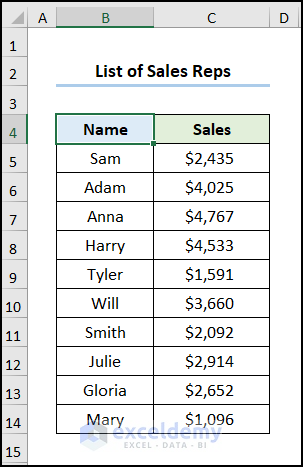
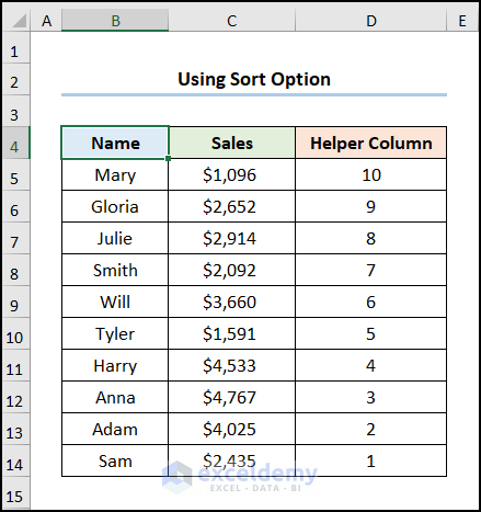
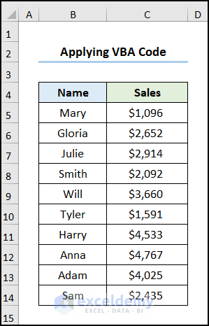
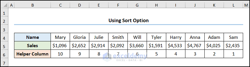
Consider the following List of Sales Reps dataset, containing the Names of some sales reps and their Sales in USD. Let’s flip the columns.
We have used Microsoft Excel 365 version, but the methods should work in most other versions.
1.1 – Using Sort Option
The most common way to flip data is with the Sort option.
Steps:
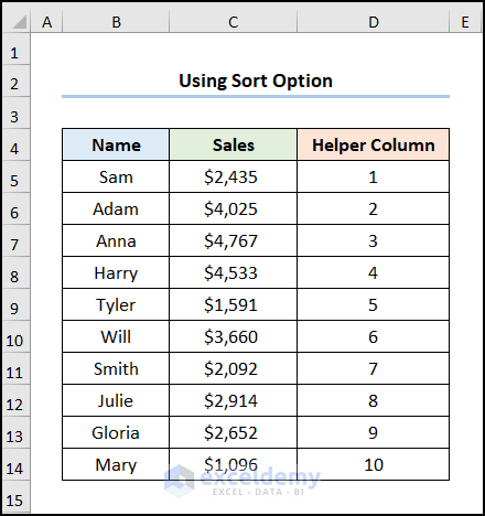
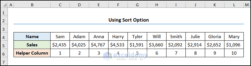
- Make a Helper Column and number it serially as shown in the picture below.
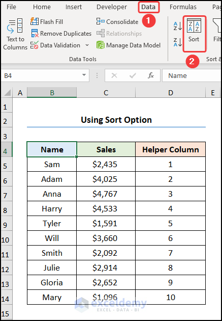
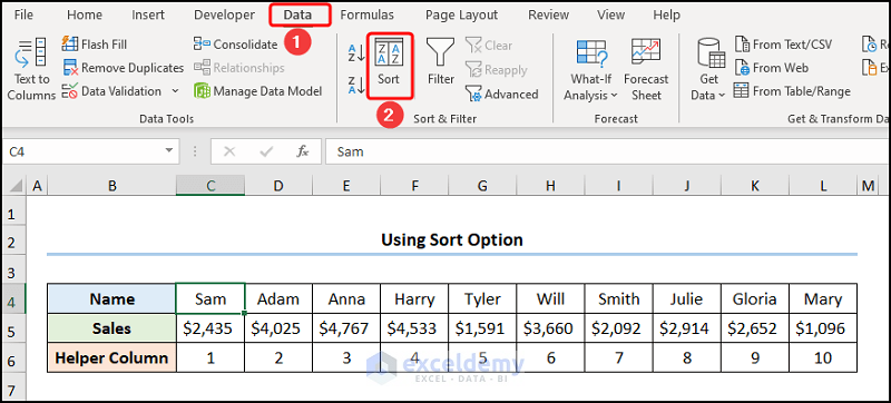
- Go to the Data tab >> click the Sort button.
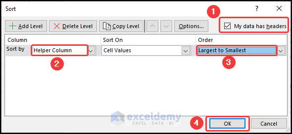
This opens the Sort window.
- Tick the My data has headers option.
- In the Sort by option, select the column heading Helper Column.
- In the Order field, choose Largest to Smallest option.
- Click OK.
This flips the table as shown in the image below.
1.2 – Using SORTBY Function
The SORTBY function sorts a range or array in ascending or descending order based on another given range or array.
Steps:
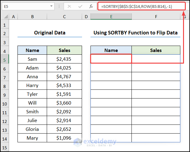
- In cell E5 enter the formula below:
=SORTBY($B$5:$C$14,ROW(B5:B14),-1)
The B5:C14 cells refer to the Name and Sales values respectively.
Formula Breakdown:
- SORTBY($B$5:$C$14,ROW(B5:B14),-1) → $B$5:$C$14 is the array argument that refers to the Names and Sales values. ROW(B5:B14) represents the by_array1 argument which returns the row numbers of the Names and Sales values. Lastly, -1 is the optional sort_order1 argument which indicates Descending order.
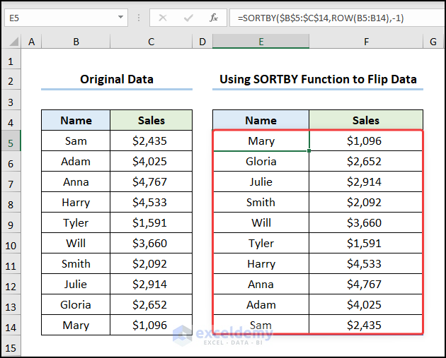
The output should look like the screenshot shown below.
1.3 – Using INDEX Function
The INDEX function returns a value according to given row and column numbers. Moreover, the INDEX function is compatible with older versions of Excel.
Steps:
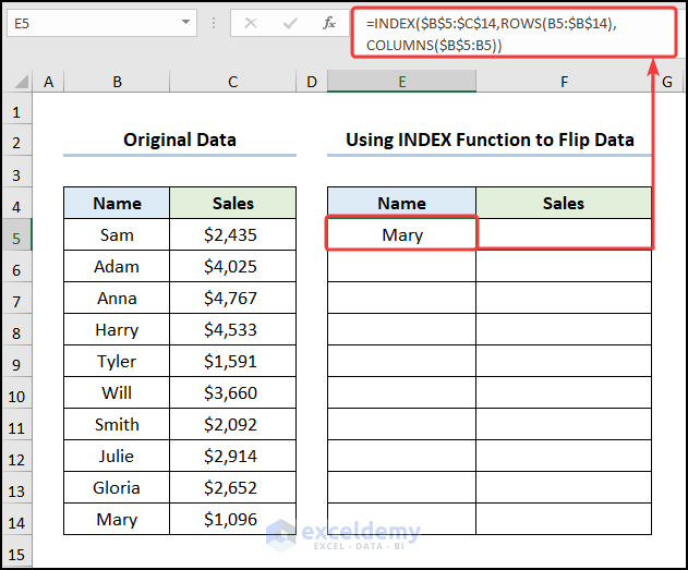
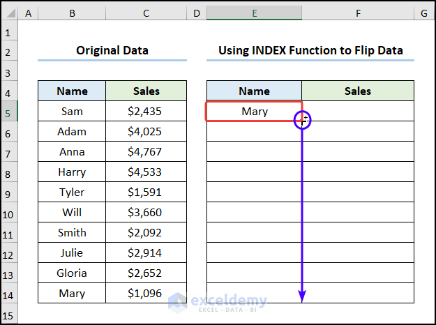
- In cell E5 enter the formula given below:
=INDEX($B$5:$C$14,ROWS(B5:$B$14),COLUMNS($B$5:B5))
The B5:C14 cells refer to the Name and Sales values respectively while the B5:B14 cells indicate the Names.
Formula Breakdown:
- INDEX($B$5:$C$14,ROWS(B5:$B$14),COLUMNS($B$5:B5)) → the $B$5:$C$14 is the array argument which is the marks scored by the students. ROWS(B5:$B$14) is the row_num argument which indicates the row location. COLUMNS($B$5:B5) is the optional column_num argument that points to the column location.
- Output → Mary
- Use the Fill Handle tool to copy the formula to the cells below.
- Select the E5:E14 range.
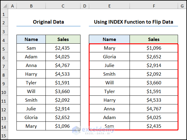
- Drag the Fill Handle Tool across to copy the formula into the adjacent cells.
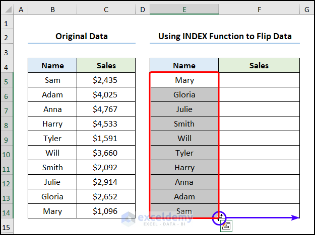
The table is flipped
1.4 – Using VBA Code
If you often need to flip the table by columns, use the VBA code below.
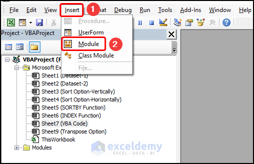
- Go to the Developer tab.
- Click the Visual Basic button.
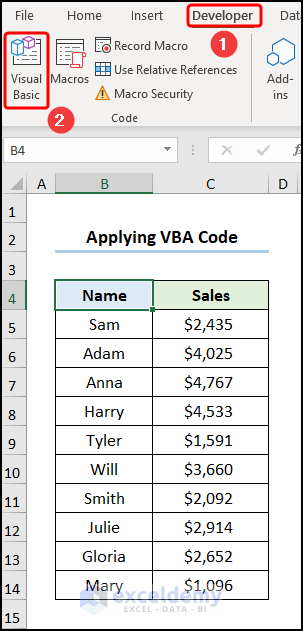
This opens the Visual Basic Editor in a new window.
- Go to the Insert tab >> select Module.
Copy the following code and paste it into the editor window:
Sub Invert_Table_By_Columns()

Dim First_row As Variant
Dim End_row As Variant
Dim First_num As Integer
Dim End_num As Integer

First_num = 1
End_num = Selection.Rows.Count

Do While First_num < End_num
First_row = Selection.Rows(First_num)
End_row = Selection.Rows(End_num)

Selection.Rows(End_num) = First_row
Selection.Rows(First_num) = End_row

First_num = First_num + 1
End_num = End_num - 1

Loop

End Sub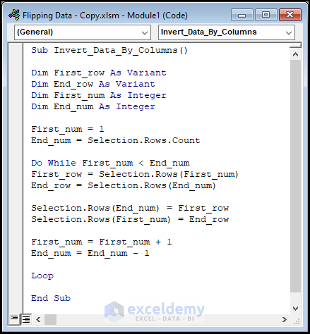
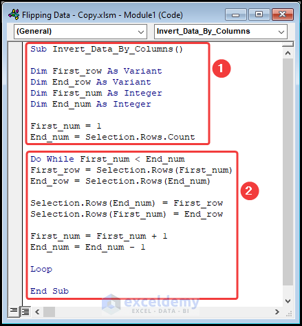
⚡ Code Breakdown:
The code is divided into 2 steps.
- In the first portion, the sub-routine is given a name, Invert_Table_By_Columns().
- We define the variables First_row, End_row, First_num, and End_num.
- We assign Variant and Integer data types to these variables respectively.
- We set First_num to 1 and use Selection.Rows.Count to obtain the End_num.
- In the second portion, we apply the Do While statement to interchange the first and the last rows.
- The loop moves to the next row and repeats this until all the rows are flipped.
- Select the B5:C14 range.
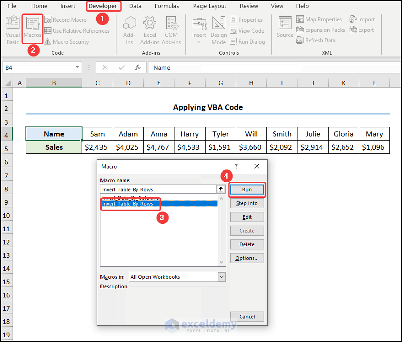
- Click the Macros button.
- Choose the Invert_Table_By_Columns macro.
- Click the Run button.
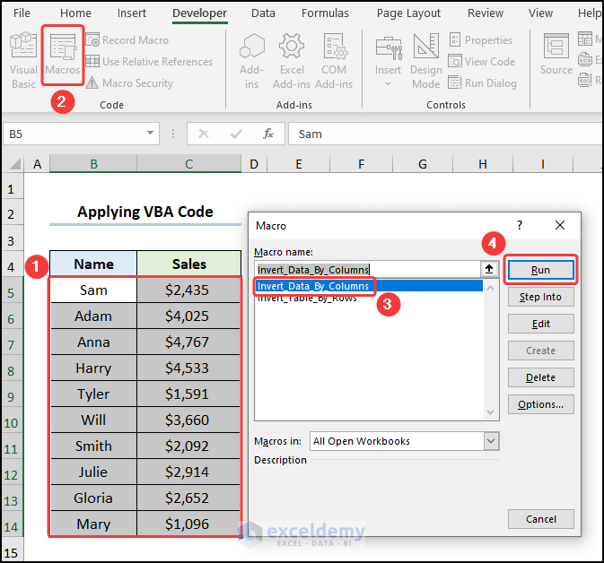
The results should look like the screenshot below.
Read More: How to Flip Data Vertically in Excel
Method 2 – Flipping Table by Rows
2.1 – Using Sort Option
Steps:
- Insert a Helper Column and number it sequentially.
- Go to the Data tab >> click the Sort button.
This opens the Sort wizard.
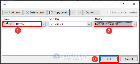
- Click the Options button >> choose the Sort left to right option.
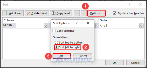
- In the Sort by option, select Row 6.
- In the Order field, choose Largest to Smallest.
- Click the OK button.
This flips the table as shown in the image below.
2.2 – Using VBA Code
Steps:
- Follow Steps 1-2 from the previous method to open the Visual Basic editor, insert a new Module and enter the code.
Sub Invert_Table_By_Rows()

    Dim r_range As Range
    Dim wk_range As Range
    Dim ar_rng As Variant
    Dim x As Integer, y As Integer, z As Integer

    On Error Resume Next

    xTitleId = "Invert_Table_Horizontally"
    Set wk_range = Application.Selection
    Set wk_range = Application.InputBox("Select a range of cells", xTitleId, wk_range.Address, Type:=8)
    ar_rng = wk_range.Formula

    Application.ScreenUpdating = False
    Application.Calculation = xlCalculationManual

    For x = 1 To UBound(ar_rng, 1)
        z = UBound(ar_rng, 2)
        For y = 1 To UBound(ar_rng, 2) / 2
            xTemp = ar_rng(x, y)
            ar_rng(x, y) = ar_rng(x, z)
            ar_rng(x, z) = xTemp
            z = z - 1
        Next
    Next

    wk_range.Formula = ar_rng
    Application.ScreenUpdating = True
    Application.Calculation = xlCalculationAutomatic
End Sub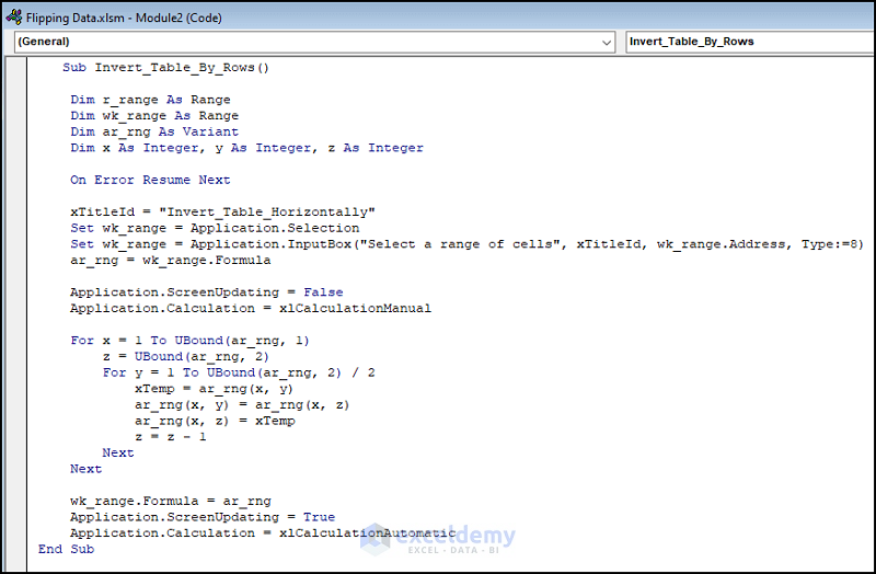
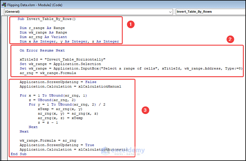
⚡ Code Breakdown:
The code is divided into 3 steps.
- In the first portion, the sub-routine is given a name, Invert_Table_By_Rows().
- We define the variables and assign Range, Variant and Integer data types respectively.
- In the second portion, an input box prompts the user to enter the range of cells to flip.
- In the third portion, we use a nested For Loop to iterate through all the values in the given range and swap their positions one by one.
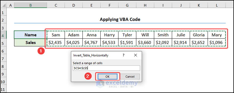
- Click the Macros button >> choose Invert_Table_By_Rows macro >> click the Run button.
- Select the C4:L5 range of cells.
- Click the OK button.
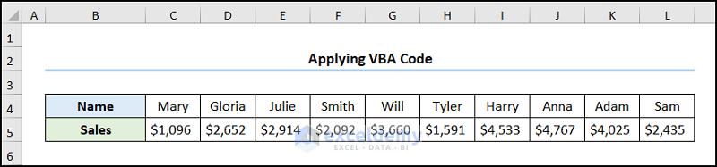
The results should look like the picture shown below.
Read More: How to Flip Data Horizontally in Excel
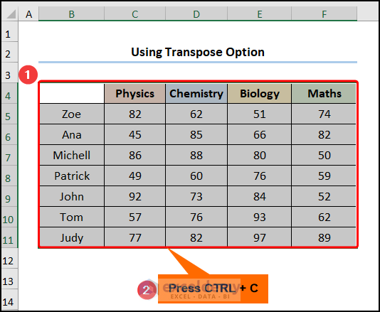
Using Transpose Option to Convert Columns to Rows
Excel allows you to convert multiple columns in a table into rows using the Transpose option.
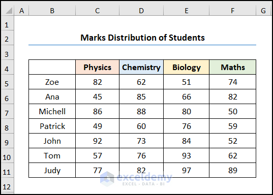
Consider the Marks Distribution of Students dataset shown in the B4:F11 cells below. Let’s transpose it.
Steps:
- Select the entire dataset, in this case, the B4:F11 range.
- Press CTRL + C on your keyboard.
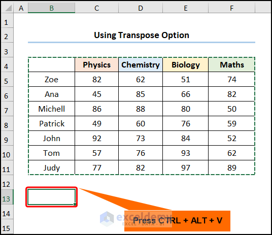
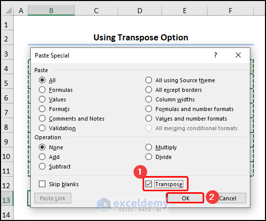
- In cell B13 press CTRL + ALT + V to open the Paste Special dialog box.
- Select the Transpose option.
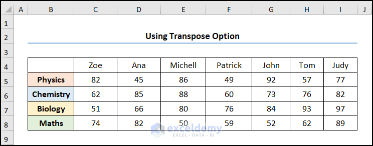
- Click the OK button.
The result should look like the image given below.
Download Practice Workbook
Related Article
- How to Flip Data in Excel Chart
- How to Mirror Data in Excel
- How to Reverse Text to Columns in Excel
- How to Reverse Column Order in Excel
- How to Reverse Data in Excel Chart
<< Go Back to Excel Reverse Order | Sort in Excel | Learn Excel
Get FREE Advanced Excel Exercises with Solutions!
